

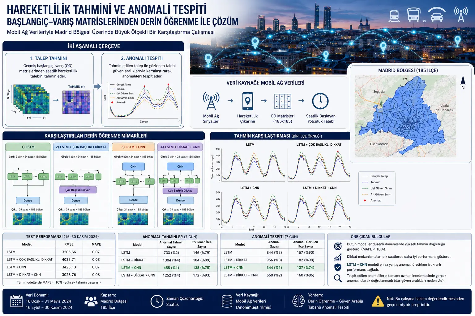
Яке аз муҳимтарин саволҳо дар transport planning чунин аст: Одамон аз кадом минтақа ба кадом минтақа, дар кадом соатҳо ва бо чӣ шиддат ҳаракат мекунанд? Ҷавоби ин савол ба бисёр соҳаҳо — аз public-transport capacity то traffic management, аз road-maintenance planning то operational decisions дар special-event days — таъсири мустақим дорад.
Ин гуна mobility information одатан бо origin-destination matrices ифода мешавад. Origin-destination matrix data structure аст, ки нишон медиҳад дар time interval муайян чанд нафар аз як минтақа ба минтақаи дигар сафар кардаанд. Масалан, агар districts-и як шаҳр дар rows ва columns ҷойгир шаванд, row origin region ва column destination region-ро ифода мекунад. Ҳар cell бошад number of trips between specific origin-destination pair-ро нишон медиҳад.
Main problem-и study ин аст, ки mobility demand аз historical data learned шуда, future demand predicted ва unusual deviations аз expected behavior detected шаванд. Anomaly дар transport system метавонад demand-и аз normal pattern фарқкунанда аз сабаби holiday, strike, sports event, weather, accident, infrastructure disruption ё unexpected social mobility бошад. Агар чунин deviations барвақт ошкор шаванд, transport operators метавонанд service frequency-ро зиёд кунанд, capacity-ро дар certain areas adjust кунанд, traffic management centers preventive action гиранд ё special-situation plans-ро activate кунанд.
Чаро ин мушкил муҳим аст?
Urban mobility random нест. Repeated patterns вуҷуд доранд: weekday morning commute, lower activity around noon, evening peak after work, different weekend tendencies ва changed travel behavior on holidays. Аммо ин patterns ҳамеша яксон намемонанд. Concert, football match, bad weather, strike ё road closure метавонад demand-ро дар certain areas хеле болотар ё пасттар аз normal кунад.
Аз perspective-и transport management савол танҳо “чанд нафар ҳаракат мекунанд?” нест. Саволи муҳимтар ин аст: “Оё нисбат ба expected demand unusual situation вуҷуд дорад ва он дар куҷо пайдо мешавад?” Зеро system метавонад дар normal day хуб кор кунад, аммо same plan дар abnormal day insufficient шавад. Агар abnormal demand пешакӣ ё дар early stage detect шавад, transport system more proactively managed шуда метавонад.
Study аз он ҷиҳат муҳим аст, ки mobility forecasting ва anomaly detection-ро дар same framework баррасӣ мекунад. Model-и танҳо good forecasting метавонад decision maker-ро location/time of anomaly нишон надиҳад. System-и only anomaly detection ҳам, агар strong expected-demand forecast надошта бошад, метавонад normal fluctuations-ро mistakenly anomaly ҳисоб кунад. Study ин ду need-ро combine намуда, аввал expected demand-ро ҳисоб мекунад ва баъд deviations-ро relative to that expectation evaluate мекунад.
Чаро mobile-network data истифода мешаванд?
Data-и study origin-destination matrices мебошанд, ки аз mobile-network data тавлид шудаанд. Mobile-network data имкон медиҳанд movement patterns аз connection-и phones бо base stations infer шаванд. Вақте ин data not for individual tracking, but to understand aggregated and anonymized mobility flows истифода мешаванд, онҳо метавонанд urban-scale data source-и хеле valuable бошанд.
Mobile-network data барои transport planning advantages-и муҳим доранд. Traditional surveys expensive, sample-limited ва period-specific мебошанд. Sensors, cameras ё turnstile data танҳо movement at certain points-ро мебинанд. Mobile-network data бошад broad area, long time period ва inter-regional movement-ро more holistically represent мекунанд.
OD matrices дар study аз ҷониби Nommon барои Ministry of Transport and Sustainable Mobility of Spain тавлид шудаанд. Mobile-network data бо Nommon Mobility Insights processed шуда, activity-travel diaries барои sampled mobile users сохта ва бо census data ба total population expanded шудаанд. Matrices на танҳо regional movement, балки rich segmentation by time of day, trip purpose, distance, age, sex, residence ва income пешниҳод мекунанд.
Literature gap чист?
Дар transport-demand forecasting ва anomaly-detection literature methods-и гуногун истифода шудаанд. Баъзе studies statistical methods истифода мекунанд. Kalman filters, Gaussian-kernel methods, Z-score criteria ва confidence intervals classical tools мебошанд. Interpretability-и онҳо high аст, аммо дар large-scale, high-dimensional OD matrices scalability problem дошта метавонанд.
Machine-learning methods барои кам кардани ин limitations истифода шуданд. Support-vector machines, random forests, k-nearest neighbors, linear models ва PCA for dimensionality reduction дар studies гуногун татбиқ шудаанд. Аммо strong anomalies ва nonstationary mobility patterns метавонанд model stability-ро таъсир диҳанд.
Deep learning, махсусан LSTM networks, барои capturing long-term dependencies in time series дар transport-demand forecasting prominent шудааст. Аммо important gap вуҷуд дорад: Most studies ё forecasting accuracy ё anomaly detection-ро focus мекунанд; systematic comparisons-и different deep-learning architectures барои both forecasting and anomaly detection on large-scale OD data маҳдуданд.
Study ҳамин gap-ро focus мекунад. Four different deep-learning architectures under same data and evaluation framework compare шудаанд. Ҳамин тавр нишон дода мешавад, ки LSTM, attention mechanism ва CNN components дар кадом conditions better work мекунанд, performance дар low demand ва peak hours чӣ гуна differ мекунад ва false-flagging behavior дар anomaly detection чӣ гуна тағйир меёбад.
Two-stage proposed method чӣ гуна кор мекунад?
Method ду stage дорад. First stage demand forecasting аст. Deep-learning time-series model past multidimensional OD demand data-ро истифода бурда, next day hourly demand-ро тавлид мекунад. Input previous nine days hourly demand аст; output бошад 24-hour demand forecast барои 185 districts мебошад. Яъне every forecast demand matrix with dimensions 185 × 24 истеҳсол мекунад.
Second stage anomaly detection аст. Дар ин stage model forecast directly as “true reference” қабул намешавад. Аввал compatibility-и forecasted demand with historical demand behavior check мешавад. Баъд actual observed demand бо validated forecast compare мешавад. Агар actual demand outside confidence interval бошад, anomaly candidate flagged мешавад.
Ин two-stage structure муҳим аст. Difference from bad forecast метавонад real anomaly барин намоён шавад. Study барои кам кардани risk аввал checks whether forecast is consistent with historical pattern. Thus system before asking “is actual demand abnormal?” first asks “is model’s expected demand plausible?”
Validation of expected demand against historical behavior
First confidence interval барои checking if forecasted demand is consistent with previous same-weekday pattern истифода мешавад. Масалан, if forecast is for Tuesday, previous Tuesdays considered мешаванд. Mean demand ва standard deviation аз ин days computed мешаванд.
Confidence interval дар study чунин аст:
\[ [(1-\alpha)avg_n-k\cdot std_n,\ (1+\alpha)avg_n+k\cdot std_n] \]
Дар ин ҷо avg_n mean demand for previous n same weekdays мебошад. std_n standard deviation of same historical observations. k parameter, ки width of confidence interval in standard-deviation units-ро муайян мекунад. n number of previous periods ва α flexibility for small fluctuations not fully captured by standard deviation мебошад.
Маънои everyday-и formula: “Дар previous similar days demand in this area roughly within what range буд? Is today’s model forecast within expected behavior band?” Агар forecast within interval бошад, historically consistent ҳисоб мешавад. Агар outside бошад, ин метавонад either real demand pattern shift or degraded model performance бошад.
Comparing actual demand with predicted demand
Пас аз он ки forecast historically plausible ҳисоб шуд, stage two actual observation-ро compare мекунад. Confidence interval this time around forecast value built мешавад:
\[ [(1-\alpha)prediction-\ell\cdot std_n,\ (1+\alpha)prediction+\ell\cdot std_n] \]
Дар ин ҷо prediction model forecast, std_n standard deviation of previous n similar days, ℓ calibration parameter controlling anomaly-detection interval width, ва α same flexibility parameter мебошад.
Actual observations within interval normal ҳисоб мешаванд. Values outside interval anomaly candidates flagged мешаванд. “Anomaly candidate” wording important аст. Study stresses every flagged value should not automatically be treated as real anomaly and expert validation is needed. Small deviations outside interval may result not from actual event but from too-narrow intervals or natural variability.
Application in Madrid Region
Method дар Madrid Region test шудааст. Region ба 185 districts divided шудааст. Study map spatial distribution-и districts-ро нишон медиҳад ва blue areas scope of analysis-ро indicate мекунанд. Map муҳим аст, зеро study not single corridor or station, but broad regional mobility data-ро истифода мекунад.
OD matrices ба hourly originating-trip demand for each district transformed шудаанд. Ҳамин тавр model simultaneously 185 district hourly-demand time series-ро forecast мекунад. Ин аз single time-series forecasting much harder аст, зеро ҳар district own rhythm дорад ва inter-regional relationships and common temporal patterns ҳам вуҷуд доранд.
Experimental dataset only full and regular weeks in 2024-ро includes мекунад. Holidays and major disruptions excluded шудаанд. Analysis period 16 January–31 May 2024 and 16 September–30 November 2024 мебошад. Easter week ва Madrid regional holiday week excluded шудаанд. Ин selection барои understanding model behavior under regular demand conditions аст; holiday/major-event periods more complex мебошанд ва future work require separate assessment.
Deep-learning architectures compared
Study four neural-network architectures compare кардааст. First baseline LSTM architecture аст. LSTM networks барои learning long-term temporal dependencies designed шудаанд. Therefore suitable for forecasting future demand from previous days/hours mobility patterns мебошанд. Baseline architecture се 128-unit LSTM layers, 0,3 dropout, 1024-neuron fully connected layer ва 24 × 185 output layer истифода мекунад.
Second model LSTM with multi-head attention мебошад. Attention mechanism allows model to put more weight on more important time steps in past observations. For example, if a district demand has informative patterns at certain hours or weekdays, attention can capture these relationships better. Here attention module with four heads, key dimension 32 and dropout 0,1 inserted between LSTM stack and dense layers.
Third model combines LSTM and CNN. CNN layer at input extracts local temporal and spatial patterns. In mobility data, neighboring or functionally connected regions can have relationships. Congestion/activity in one region may affect demand in another. CNN helps extract such short-term/local patterns. Model adds convolution layer with 64 filters and kernel size 5 to baseline LSTM architecture.
Fourth model combines LSTM, multi-head attention and CNN. Most complex architecture includes convolution layer, three LSTM layers, multi-head attention module, global average pooling and dense output layers. Goal is to combine CNN local-pattern extraction, LSTM long-term dependency learning and attention focus on important time steps.
Training and test setup
All models were trained with MAE loss and optimized with Adam. Dataset was split into training and test subsets. Training set included all observations up to 14 November 2024. Test set covered subsequent 16 days, 15–30 November 2024, used only for generalization evaluation.
Input-output examples created using nine-day sliding window. Model looks at previous nine days hourly demand and predicts 24-hour demand for one day. Each forecast contains 185 districts × 24 hours, so output matrix is 185 × 24.
Performance evaluated with RMSE and MAPE. RMSE penalizes large errors more, thus making large deviations in high-demand periods more visible. MAPE measures relative error against observed value; in low-demand periods small absolute differences can create large percentage errors. Thus using both metrics is important.
RMSE ва MAPE чӣ маъно доранд?
Гарчанде formulas дар source explicitly дода нашудаанд, basic relationships барои understanding used metrics чунинанд. These formulas are background formulas for explaining study logic:
\[ RMSE=\sqrt{\frac{1}{N}\sum_{i=1}^{N}(y_i-\hat{y}_i)^2} \]
Дар ин ҷо y_i actual demand, \hat{y}_i predicted demand ва N total observations мебошанд. Because RMSE squares errors, it is more sensitive to large errors. Large error at peak hours is strongly penalized.
\[ MAPE=\frac{100}{N}\sum_{i=1}^{N}\left|\frac{y_i-\hat{y}_i}{y_i}\right| \]
Дар ин ҷо MAPE error as percentage of actual value медиҳад. At low demand, small absolute deviation may become high percentage error. Study uses different sensitivity of RMSE and MAPE to explain why attention models work well at peaks but weaker at low demand.
Forecasting results: Which model performed best?
Four model error values on test set:
| Model | RMSE | MAPE |
|---|---|---|
| LSTM | 3205,66 | 0,07 |
| LSTM + multi-head attention | 4033,71 | 0,08 |
| LSTM + CNN | 3423,13 | 0,07 |
| LSTM + multi-head attention + CNN | 3028,76 | 0,08 |
Ҳама models high forecasting performance нишон доданд. All MAPE values 0,07–0,08 range буданд; relative error below 10 percent. Ин нишон медиҳад, ки under regular operating periods mobility demand can be accurately forecast with deep-learning models.
Lowest RMSE 3028,76 from LSTM + multi-head attention + CNN model буд. This shows strong performance in reducing large deviations especially during high-demand periods. However same model MAPE is 0,08, suggesting weaker relative performance at low-demand hours. Baseline LSTM and LSTM-CNN have better MAPE of 0,07.
Important interpretation: Attention models capture peak-demand hours better, but may perform worse during low demand. Simpler models without attention better represent low-demand hours but may be more limited in capturing three daily peaks. Therefore “best model” depends on application. If peak-hour forecasting is priority, attention models may be advantageous. If stable relative errors and fewer false anomalies during low demand are priority, simpler LSTM or LSTM-CNN may be preferable.
What do forecast-curve figures show?
Forecast comparison graphs show actual demand and forecast curves of four models for a representative district. Daily mobility has clear wave structure: low demand at night/early morning, rising activity during day and peaks at certain hours.
Graphs show all models capture general daily pattern. However systematic differences appear. Models without attention are closer during low-demand hours but struggle more to capture peak magnitude. Attention models represent peak hours more accurately, but relative deviations increase at low demand.
Important point is not only visual confirmation of error table, but showing different hours have different difficulty. A model can perform strongly at peak demand yet over/underpredict at night. This becomes critical in anomaly detection because low-variability hours have narrow confidence intervals and small deviations can be falsely flagged.
Натиҷаҳои anomaly detection
Дар study hourly forecasts for 185 districts over seven-day analysis evaluated шудаанд. Total number of forecasts 31.080 мебошад. Барои ҳар model abnormal-forecast counts ва number of affected districts чунинанд:
| Model | Abnormal forecast count | Number of districts with abnormal forecasts |
|---|---|---|
| LSTM | 733 (%2) | 146 (%79) |
| LSTM + multi-head attention | 1304 (%4) | 184 (%99) |
| LSTM + CNN | 455 (%1) | 138 (%75) |
| LSTM + multi-head attention + CNN | 1252 (%4) | 172 (%93) |
Table нишон медиҳад, ки LSTM-CNN smallest number of abnormal forecasts produced кардааст. Models with multi-head attention more abnormal forecasts produced. Ин situation especially to weaker relative performance at low demand and narrow confidence intervals linked шудааст.
Дар next stage, values flagged as anomalies relative to actual observed demand evaluated шудаанд:
| Model | Number of anomalies | Number of districts with anomalies |
|---|---|---|
| LSTM | 844 (%3) | 167 (%90) |
| LSTM + multi-head attention | 956 (%3) | 182 (%98) |
| LSTM + CNN | 344 (%1) | 137 (%74) |
| LSTM + multi-head attention + CNN | 660 (%2) | 160 (%86) |
Дар ин ҷо ҳам LSTM-CNN best anomaly-detection behavior produced кардааст. Model 344 anomalies flagged кард, significantly fewer false flags than other models. Interpretation ин аст, ки LSTM-CNN long-term temporal-dependency learning of LSTM ва CNN short-term/spatial pattern extraction-ро combine карда, more stable forecasts and reliable confidence intervals медиҳад.
Оё detected anomalies real anomalies буданд?
Study як very important result дорад: None of detections in analyzed test set were judged to be true anomalous events. Flagged values valid demand observations буданд. Anomaly-like appearance mostly caused by confidence intervals being too narrow.
Вақте confidence interval narrow аст, actual demand ҳатто агар very close to normal behavior бошад ҳам, метавонад outside interval барояд. Ин especially when previous days’ demand variability is very low occurs. Standard deviation small бошад, std_n term confidence band-ро narrow мекунад. Thus small fluctuations can be flagged as statistical anomaly candidates.
Figures show abnormal forecasts and detected anomalies close to confidence interval boundaries. This supports interpretation that these are not real transport disruptions or large demand shifts, but mostly calibration-sensitivity issues.
Чаро Bollinger-band-like confidence intervals бояд carefully calibrated шаванд?
Confidence intervals in study as variation of Bollinger band approach built шудаанд. Because based on mean and standard deviation, method interpretable and practical аст. Аммо standard deviation low бошад, interval too narrow; high бошад, interval too wide and true anomalies might be missed.
Therefore parameter calibration supported by expert validation. Nommon mobility experts inspected time series of detected events and evaluated whether true anomaly. Final selected structure used moving average of six periods, k = ℓ = 2 standard-deviation coefficient and α = 1 flexibility parameter. This configuration reported as suitable balance between sensitivity and robustness.
Study also observed wider confidence intervals on Fridays. One reason is that historical sample included 1 November, an official holiday in Spain. Holiday increased variability in historical Friday pattern and widened confidence band for later Fridays. This detail shows calendar effects are important in anomaly detection.
Таъсир ба ҳаёти ҳаррӯза чӣ буда метавонад?
Such a system can provide many practical benefits in city management. For example, if public-transport operator detects more originating trips than expected in a district at certain hours, it can plan additional service or redirect vehicles. Traffic-management center can investigate whether unusually high mobility is due to event, accident or weather. In long term, planners can understand regular and irregular urban mobility patterns and strengthen infrastructure/service decisions.
Approach is useful not only for crisis days but also for understanding normal days better. If model reliably forecasts regular periods, unusual periods become easier to identify. In other words, defining “normal” well is prerequisite for detecting “abnormal” correctly.
Ҷиҳатҳои қавии study
One strength is use of large-scale, high-dimensional mobility data. Hourly demand forecasting for 185 districts is not single road or small OD pair. This scale means method tested on problem closer to real regional transport planning.
Second strength is systematic comparison of four deep-learning architectures. Using baseline LSTM as reference makes contribution of attention mechanism and CNN components clearer. Study does not simply say “most complex model is best”; it shows model choice can depend on peak-demand, low-demand and anomaly-detection objectives.
Third strength is inclusion of human expert validation. Anomaly detection not left entirely automatic; flagged values were interpreted with mobility experts. This is important in transport planning where detections can lead to operational decisions.
Маҳдудиятҳои study
Most important limitation is experimental dataset selected from regular weeks. Holidays, major disruptions and significant irregularities were specifically excluded. This is suitable for understanding normal-condition forecasting and false-anomaly behavior, but does not directly show performance during periods rich in true anomalies.
Second limitation is that detected anomalies in test week did not correspond to real anomaly. This is useful for understanding false positives, but to measure true-event detection success more irregular datasets containing events are needed.
Third limitation is incomplete integration of exogenous variables in anomaly interpretation. Study proposes future integration of weather, event data, calendar effects and other external factors. Without this integration, system can flag deviation but has limited capacity to explain its cause automatically.
Fourth, study is preprint and not peer reviewed. Results should be seen as valuable technical comparison, not final validated scientific evidence or application standard.
Study чӣ мегӯяд ва чӣ намегӯяд?
Study shows that hourly mobility demand in Madrid Region can be forecast with high accuracy using deep-learning models and OD matrices derived from mobile-network data. In regular periods all models have MAPE below 10 percent. It also shows LSTM-CNN as stable choice producing fewer false flags in anomaly detection.
Study does not say all anomalies will certainly be detected in real irregular events. It does not claim a directly deployment-ready real-time product. It does not guarantee mobile-network data have same quality/coverage in every city. Automatic classification of anomaly causes is not main scope; future integration of weather and event data is suggested.
Усул ва Натиҷаҳои Таҳқиқот
Қадамҳои усул
- Data source: Origin-destination matrices generated from mobile-network data were used.
- Study area: Madrid Region divided into 185 districts.
- Demand series: OD matrices converted to hourly originating-trip demand, yielding 185 parallel hourly time series.
- Data selection: Regular and complete weeks in 2024 selected; holidays and major disruption periods excluded.
- Input-output structure: Previous nine days hourly demand used to predict next day’s 24-hour demand.
- Model comparison: LSTM, LSTM + multi-head attention, LSTM + CNN, and LSTM + multi-head attention + CNN tested.
- Performance measurement: Forecast performance evaluated with RMSE and MAPE.
- Anomaly detection: Forecasts and observations compared with Bollinger-band-like confidence intervals.
- Expert validation: Detected deviations reviewed with mobility experts and calibration assessed accordingly.
Формулаҳои асосӣ
| Formula | Explanation |
|---|---|
| [ [(1-\alpha)avg_n-k\cdot std_n,\ (1+\alpha)avg_n+k\cdot std_n] ] | Confidence interval checking whether forecast is consistent with historical same-weekday behavior. |
| [ [(1-\alpha)prediction-\ell\cdot std_n,\ (1+\alpha)prediction+\ell\cdot std_n] ] | Anomaly-detection interval determining whether actual observed demand remains within normal range around forecast. |
| [ RMSE=\sqrt{\frac{1}{N}\sum_{i=1}^{N}(y_i-\hat{y}_i)^2} ] | Background formula for RMSE used in study; penalizes large errors more strongly. |
| [ MAPE=\frac{100}{N}\sum_{i=1}^{N}\left|\frac{y_i-\hat{y}_i}{y_i}\right| ] | Background formula for MAPE used in study; expresses error as percentage of observed value. |
Forecast performance
| Model | RMSE | MAPE | Interpretation |
|---|---|---|---|
| LSTM | 3205,66 | 0,07 | Strong general performance; good relative error in low-demand periods. |
| LSTM + multi-head attention | 4033,71 | 0,08 | Useful for capturing peak periods; relative error can rise during low-demand hours. |
| LSTM + CNN | 3423,13 | 0,07 | Balanced performance in forecasting accuracy and anomaly-detection stability. |
| LSTM + multi-head attention + CNN | 3028,76 | 0,08 | Lowest RMSE; strong at high demand, but higher MAPE at low demand. |
Abnormal forecasts and anomaly detection
| Model | Abnormal forecast | Anomaly | Technical interpretation |
|---|---|---|---|
| LSTM | 733 | 844 | Good overall forecast, but more confidence-band flags than LSTM-CNN. |
| LSTM + multi-head attention | 1304 | 956 | More false flags due to relative deviations during low-demand hours. |
| LSTM + CNN | 455 | 344 | Fewest false anomalies and most balanced anomaly-detection model. |
| LSTM + multi-head attention + CNN | 1252 | 660 | Strong RMSE but less stable than LSTM-CNN for anomaly detection. |
Main results conveyed by figures and tables
Map dividing Madrid Region into districts shows regional scale and 185 spatial units. This demonstrates method tested not on small laboratory dataset but on high-dimensional data close to real regional mobility structure.
Forecast comparison graphs show all models capture daily demand wave, but attention models represent peak hours better, while models without attention represent low-demand hours better. This is consistent with RMSE and MAPE results.
In abnormal-forecast and anomaly graphs, flagged points appear very close to confidence-interval boundaries. This visual result supports text interpretation: detections in test week were not true anomalies, but small deviations caused by narrow confidence intervals.
Tables clearly show LSTM-CNN as advantageous architecture for anomaly detection. It maintained forecasting accuracy while reducing false anomaly flags.
Умумии technical result
Main technical conclusion is that deep-learning architectures show strong performance for large-scale mobility demand forecasting, but model selection should depend on application objective. If peak demand is priority, attention-based architectures are advantageous. If stable relative error and fewer false anomalies during low demand are important, hybrid architectures without attention such as LSTM-CNN may provide more balanced results.
For anomaly detection, findings show good forecasting alone is insufficient. Confidence-band width, historical variability, calendar effects and expert validation directly affect detection success. Therefore study proposes safer operational approach combining automated anomaly detection with human expert validation.
Ёддошт оид ба Манбаъ ва Усул
Ин мақола дар асоси таҳқиқоти Raquel Sánchez-Cauce, Oliva G. Cantú Ros, Miguel Picornell, Pablo Ruiz ва Sergio Teso бо унвони “Mobility Demand Forecasting and Anomaly Detection from Origin–Destination Matrices: A Benchmark of Deep Learning Architectures” таҳия шудааст. Authors are affiliated with Nommon Solutions and Technologies. Study is part of CONDUCTOR project funded under European Union Horizon Europe programme.
Source text is preprint research paper on SSRN. It explicitly states “This preprint research paper has not been peer reviewed”, therefore it has not passed peer review. Results should be read as technically detailed but unreviewed preprint findings, not finally validated journal evidence.
Content is based on PDF study. No claims of field-application guarantee, commercial success, certain real-time performance, generalizability to all cities or guaranteed detection of all anomalies have been added. Method uses OD matrices derived from mobile-network data, deep-learning time-series forecasting and confidence-interval-based anomaly detection.
Study tested regular weeks; holidays and major-disruption periods were excluded. Therefore method was evaluated for forecast accuracy and false-anomaly behavior under regular demand conditions. Performance during irregular periods with actual anomalies requires further testing. Stronger integration of exogenous variables such as weather, event data and calendar effects is identified as future work.
Шарҳ гузоред
Нишонии почтаи электронии шумо нашр намешавад. Майдонҳои ҳатмӣ бо * нишон дода шудаанд