

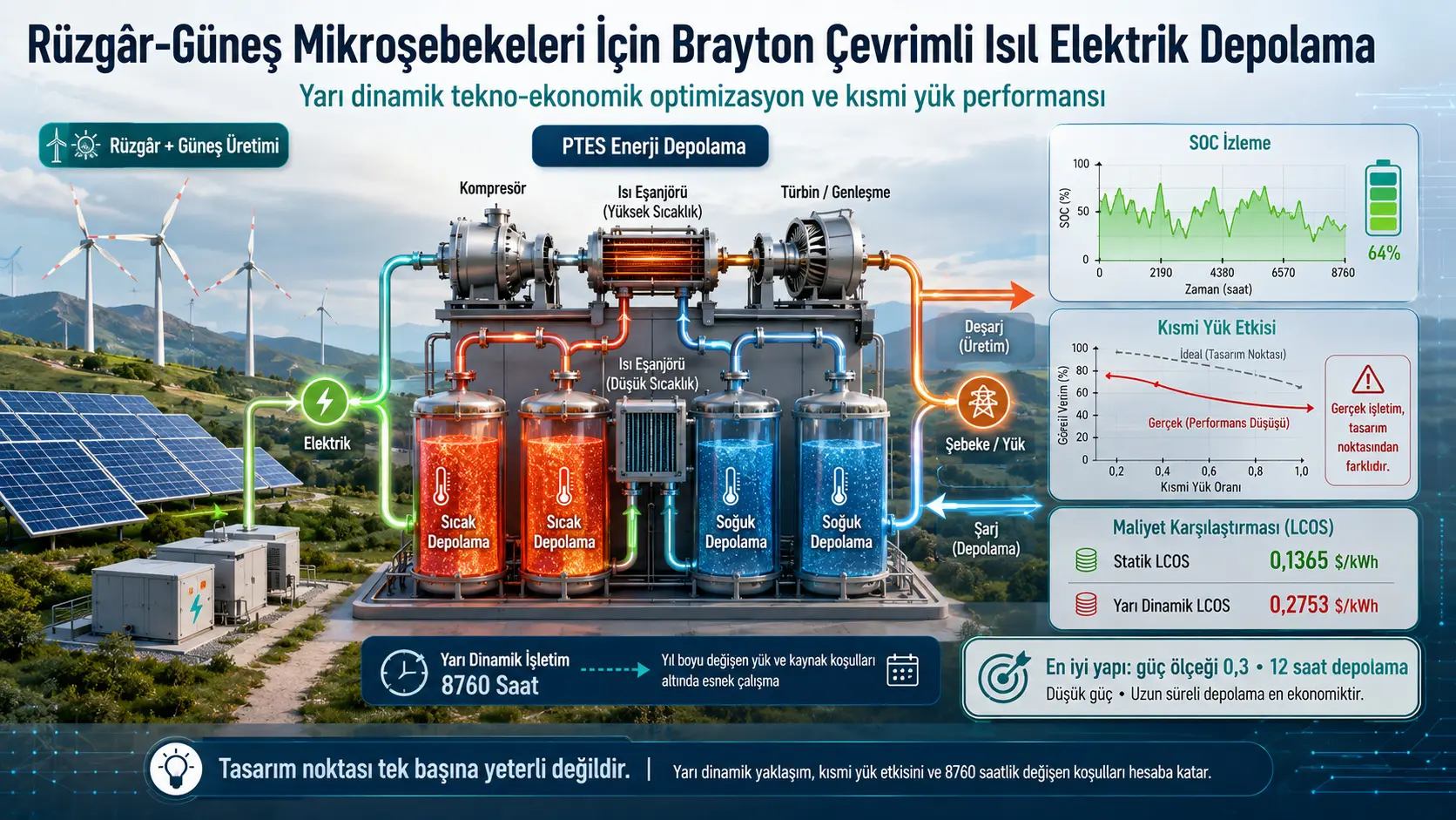
Ин таҳқиқот меомӯзад, ки тағйирёбии соатбайъии тавлиди бод ва офтоб чӣ гуна performance-и воқеии системаи pumped thermal electricity storage бо Brayton cycle-ро тағйир медиҳад. Системаи баррасишуда нерӯи барқи изофиро тавассути як heat-pump cycle-и CO₂-based дар molten salt-и ҳарорати баланд ва маҳлули ethylene glycol-и ҳарорати паст захира мекунад; ҳангоми ба вуҷуд омадани норасоии нерӯи барқ, гармии захирашударо тавассути Brayton heat-engine cycle дубора ба нерӯи барқ табдил медиҳад.
Researchers модели 8.760-соатаи quasi-dynamic operation сохтанд, ки 300 MW wind ва 300 MW photovoltaic generation-и минтақаи Qinghai-и China, local consumption бо 70 MW peak load, 80 MW external-grid transfer limit, state of charge-и storage tank ва part-load losses-и compressor ва expander-ро якҷо мекунад. Reference system-и ибтидоӣ 100 MW discharge power ва six hours storage duration дорад.
Дар fixed design-point approach annual discharged electricity 219,00 GWh, round-trip efficiency %66,92 ва levelized cost of storage 0,1365 USD/kWh ҳисоб шуд. Вақте real-time chronological operation, SOC limits ва part-load degradation ба назар гирифта шуданд, annual discharge то 94,20 GWh ва dynamic round-trip efficiency то %55,81 кам шуд; LCOS бошад то 0,2753 USD/kWh боло рафт. Ҳамин тавр, static assessment дар ин scenario realistic cost-ро тақрибан %101,67 кам нишон додааст.
Вақте power ва energy capacity якҷо optimized шуданд, most economical wind-solar hybrid configuration бо power scale баробар ба %30 reference power ва 12-hour storage duration ба даст омад. Барои ин configuration charge ва discharge powers respectively approximately 44,8 MW ва 30,0 MW, dynamic efficiency %64,37 ва LCOS 0,1772 USD/kWh буданд. Results нишон медиҳанд, ки сохтани system-и калон барои гирифтани highest instantaneous renewable-energy surplus на ҳамеша most economical solution аст.
Шарҳи муфассал
Масъалаи асосии таҳқиқот чист?
Wind ва solar power generation вобаста ба соати рӯз, weather conditions ва season пайваста тағйир меёбанд. Local electricity demand ҳамон temporal pattern-ро пайравӣ намекунад. Агар renewable generation аз total power-и local load ва power-и ба external grid интиқолшаванда зиёд шавад, қисми usable energy curtailed мешавад ё cut off мегардад. Дар соатҳое, ки generation аз local demand камтар аст, electricity deficit ба вуҷуд меояд.
Energy storage system метавонад energy-ро байни ин ду period интиқол диҳад. Аммо танҳо nominal power, storage duration ва design-point efficiency-и storage-ро дидан кофӣ нест. Economic ва thermodynamic performance-и system аз conditions-и зерин якҷо таъсир мегирад:
- Renewable-energy surplus дар кадом соатҳо ва дар кадом power levels пайдо мешавад,
- Андоза ва duration-и local electricity deficit,
- Оё storage tank дар он лаҳза пур ё холӣ аст,
- Charge ва discharge equipment нисбат ба nominal power дар кадом load кор мекунад,
- Compressor ва expander дар part load чӣ қадар efficiency аз даст медиҳанд,
- Installed capacity дар тӯли сол то чӣ андоза истифода мешавад.
Main research question чунин аст: PTES system-и пайваст ба wind-solar microgrid, вақте дар тӯли сол under real chronological constraints operate мекунад, аз design-point calculations то чӣ андоза дур мешавад ва matching-и power ва storage duration чӣ гуна бояд тағйир дода шавад?
Pumped thermal electricity storage чист?
Pumped thermal electricity storage ё PTES як long-duration storage technology аст, ки electricity-ро аввал ба hot ва cold energy ва баъдан боз ба electricity табдил медиҳад. Ба ҷойи electrochemical storage мисли batteries, он аз temperature difference байни hot ва cold storage media истифода мебарад.
System-и таҳқиқшуда ба closed CO₂ Brayton cycle асос ёфтааст. High-temperature storage medium як four-component molten salt бо broad liquid temperature range, ва low-temperature storage medium ethylene glycol-water solution мебошад.
Charge cycle
Figure 1(a) charge cycle-ро нишон медиҳад, ки ҳангоми зиёд шудани wind ва solar generation аз power-и қабулшавандаи microgrid ба амал меояд:
- Electricity with curtailment risk compressor-ро тавассути motor ба кор меандозад.
- CO₂ compressed шуда, ба high pressure ва temperature мерасад.
- CO₂ дар high-temperature heat exchanger heat-ро ба molten salt медиҳад.
- Regenerator қисми heat-и дохили cycle-ро recover мекунад.
- Cold energy тавассути expander ва low-temperature heat exchanger stored мешавад.
- Electrical energy дар шакли hot molten salt ва cooled ethylene glycol solution stored мешавад.
Ҳангоми charge, hot-storage side аз high-temperature hot tank ва low-temperature hot tank; cold-storage side аз high-temperature cold tank ва low-temperature cold tank истифода мебарад.
Discharge cycle
Figure 1(b) discharge cycle-ро нишон медиҳад, ки вақте local electricity demand аз wind-solar generation зиёд мешавад:
- CO₂ аввал дар compressor compressed мешавад.
- Он тавассути regenerator ва high-temperature heat exchanger heat-ро аз hot molten salt мегирад.
- High-temperature CO₂ аз expander гузашта mechanical power истеҳсол мекунад.
- Expander generator-ро ба кор меандозад ва electricity истеҳсол мешавад.
- CO₂ тавассути air cooler ва low-temperature heat exchanger cycle-ро complete мекунад.
Ҳамин тавр renewable-energy surplus ба соати дигар интиқол ёфта, метавонад қисми local load deficit-ро пӯшонад.
Чаро system аз ҷиҳати geographic flexibility мувофиқ ҳисобида мешавад?
PTES мисли pumped-storage hydropower ҳатман ба large elevation differences ё мисли compressed-air storage ба special underground geology ниёз надорад. Capacities-и power-conversion equipment ва thermal-storage tanks метавонанд то андозае separately интихоб шаванд. Ин feature имкон медиҳад different power ва storage-duration combinations сохта шаванд.
Аммо PTES танҳо аз storage tanks иборат нест. Compressor, expander, motor, generator, heat exchangers, regenerator, air cooler ва circulation equipment бояд якҷо кор кунанд. Аз ин рӯ low utilization ratio ва part-load operation метавонанд system cost-ро ба таври ҷиддӣ таъсир диҳанд.
Basic design values-и reference system кадомҳоянд?
| Parameter | Reference value |
|---|---|
| Nominal net discharge power | 100 MW |
| Storage duration | 6 hours |
| Nominal charge power | Approximately 149,34 MW |
| Working fluid | CO₂ |
| Hot storage medium | Four-component molten salt with broad liquid temperature range |
| Cold storage medium | Ethylene glycol solution |
| Ambient temperature | 298,15 K |
| Ambient pressure | 0,101 MPa |
| Maximum molten-salt temperature | 920 K |
| Heat-exchanger terminal temperature difference | 5 K |
| Heat-exchanger pressure-loss coefficient | 0,01 |
| Compressor isentropic efficiency | 0,90 |
| Expander isentropic efficiency | 0,90 |
| Charge-cycle compressor pressure ratio | 8 |
| Discharge-cycle compressor pressure ratio | 6 |
| Low-temperature hot-tank temperature | 630 K |
| High-temperature cold-tank temperature | 400 K |
| Design-point charge COP | 1,461 |
| Design-point heat-engine efficiency | %45,84 |
| Design-point round-trip efficiency | %66,92 |
Чаро molten salt properties муҳиманд?
Storage tank volume ва heat-exchanger design аз density, specific heat capacity, viscosity ва usable temperature range-и molten salt вобастаанд. Вақте temperature-и salt дар study аз 200 °C то 650 °C боло меравад, density аз approximately 2.078 kg/m³ то 1.604 kg/m³ кам мешавад; viscosity аз 10,4 mPa·s то 1,26 mPa·s паст мешавад.
Specific heat capacity бо temperature nonlinear тағйир меёбад ва 0,509 kJ/(kg·K) at 200 °C ва 1,706 kJ/(kg·K) at 650 °C дода шудааст. Model ин temperature-dependent properties-ро дар thermodynamic calculations истифода мебарад.
Basic thermodynamic equations кадомҳоянд?
Compressor
Isentropic efficiency-и compressor:
\[ \eta_{\mathrm{com}} = \frac{h_{\mathrm{com,out,is}}-h_{\mathrm{com,in}}} {h_{\mathrm{com,out}}-h_{\mathrm{com,in}}} \]
- ηcom: compressor isentropic efficiency,
- hcom,in: compressor inlet specific enthalpy, kJ/kg,
- hcom,out,is: isentropic outlet specific enthalpy, kJ/kg,
- hcom,out: actual outlet specific enthalpy, kJ/kg.
Compressor power:
\[ W_{\mathrm{com}} = \dot{m}_{\mathrm{com}} \left( h_{\mathrm{com,out}}-h_{\mathrm{com,in}} \right) \]
Дар ин ҷо ṁcom CO₂ mass flow rate ва Wcom power consumed by compressor-ро ифода мекунад.
Expander
Isentropic efficiency-и expander:
\[ \eta_{\mathrm{exp}} = \frac{h_{\mathrm{exp,in}}-h_{\mathrm{exp,out}}} {h_{\mathrm{exp,in}}-h_{\mathrm{exp,out,is}}} \]
Generated power:
\[ W_{\mathrm{exp}} = \dot{m}_{\mathrm{exp}} \left( h_{\mathrm{exp,in}}-h_{\mathrm{exp,out}} \right) \]
Heat exchanger
Energy balance байни hot ва cold fluids:
\[ \dot{m}_{h} \left( h_{h,\mathrm{in}}-h_{h,\mathrm{out}} \right) = \dot{m}_{c} \left( h_{c,\mathrm{out}}-h_{c,\mathrm{in}} \right) \]
Heat-exchanger pressure-loss coefficient:
\[ f_p = \frac{\Delta p}{p_{\mathrm{in}}} \]
Азбаски temperature change дар real fluids linear нест, heat exchangers ба equal-enthalpy elements тақсим шудаанд. Дар ҳар node fluid temperatures аз REFPROP database ҳисоб шуда, minimum approach temperature дар тамоми heat exchanger санҷида шудааст. Ин method барои пешгирии physically impossible temperature crossovers истифода шудааст.
Storage tank
Storage tank volume:
\[ V_{\mathrm{tank}} = \frac{\dot{m}_{s}t}{\rho} \]
- Vtank: tank volume, m³,
- ṁs: mass flow rate of storage medium, kg/s,
- t: charge or discharge duration, s,
- ρ: density of storage medium, kg/m³.
Economic model ба кадом assumptions такя мекунад?
Equipment costs барои compressor, expander, heat exchangers, storage tanks, motor ва generator бо literature-based cost functions ҳисоб шудаанд. Costs аз different years бо Chemical Engineering Plant Cost Index, ки барои 2021 ҳамчун 699,97 қабул шудааст, update шудаанд:
\[ Z_k = Z_{\mathrm{original}} \left( \frac{\mathrm{CEPCI}_{2021}} {\mathrm{CEPCI}_{\mathrm{original}}} \right) \]
Total purchased-equipment cost:
\[ Z_{\mathrm{PC}} = \sum_{k=1}^{n} Z_k \]
Economic assessment assumptions:
- Plant life: 30 years,
- Discount rate: %10,
- Annual operation and maintenance cost: %3 of total capital cost,
- Electricity cost: 0,025 USD/kWh,
- 365 full charge-discharge cycles per year in static model.
Round-trip efficiency ва LCOS чӣ гуна defined шудаанд?
Design-point round-trip efficiency ratio-и net electricity obtained during discharge ба net electricity consumed during charge мебошад:
\[ \chi = \frac{ \dot{m}_{\mathrm{dis}}t_{\mathrm{dis}} \left( W_{\mathrm{dis,exp}}-W_{\mathrm{dis,com}} \right) }{ \dot{m}_{\mathrm{chr}}t_{\mathrm{chr}} \left( W_{\mathrm{chr,com}}-W_{\mathrm{chr,exp}} \right) } \]
Levelized cost of storage:
\[ \mathrm{LCOS} = \frac{ \mathrm{FCR}\cdot Z+ \mathrm{O\&M}+ E_{\mathrm{in}}P_{\mathrm{elc}} }{ E_{\mathrm{out}} } \]
- FCR: fixed annual capital-recovery rate,
- Z: total investment cost,
- O&M: annual operation and maintenance cost,
- Ein: annual charge electricity, kWh,
- Pelc: unit electricity cost,
- Eout: annual discharge electricity, kWh.
LCOS нишон медиҳад, ки барои ҳар kilowatt-hour discharge electricity чӣ қадар investment, maintenance ва energy cost рост меояд. Вақте annual discharge amount кам мешавад, fixed investment cost ба energy-и камтар тақсим шуда, LCOS боло меравад.
Thermodynamic ва economic models чӣ гуна validated шуданд?
Thermodynamic model тавассути recalculation ва comparison бо previously published low- ва high-temperature supercritical CO₂ PTES systems validated шуд. Барои low-temperature system, round-trip efficiency source value %60,04 ва model value %59,86; барои high-temperature system source value %78,40 ва model value %78,24 буданд. Relative differences respectively approximately %0,3 ва %0,2 мебошанд.
Economic model бо another PTES study comparison шуд. LCOS дар source 0,243 USD/kWh ва дар ин model 0,248 USD/kWh ҳисоб шуд, relative difference %2,06 буд.
Ин comparisons нишон медиҳанд, ки model reference studies-ро approximately reproduce карда метавонад. Аммо validation маънои онро надорад, ки 8.760-hour operation-и ин study бо experimental ё commercial PTES plant comparison шудааст.
Wind-solar microgrid чӣ гуна modeled шудааст?
Case scenario typical wind ва solar resources дар Qinghai, China-ро ифода мекунад. Total installed renewable power 600 MW аст:
- Wind: 300 MW,
- Photovoltaic: 300 MW.
Hourly wind ва solar generation аз MERRA-2 meteorological reanalysis data derived шуда, ба UTC+8 time zone adjusted шудааст. Local consumption бо synthetic daily profile, ки industrial base load dominant аст, represented шудааст. Peak load 70 MW ва барои small operational fluctuations %3 random disturbance илова шудааст.
Maximum external-grid transfer power 80 MW аст. Ин limit mandatory export schedule нест. Аз ин рӯ PTES на барои compensation кардани hours where 80 MW cannot be exported, балки асосан барои covering local load deficit discharge мекунад.
Renewable-energy surplus ва local deficit чӣ гуна ҳисоб мешаванд?
Total power that microgrid can accept in one hour:
\[ P_{\mathrm{acc}}(t) = P_{\mathrm{demand}}(t)+P_{\mathrm{export}} \]
Total renewable generation:
\[ P_{\mathrm{RE}}(t) = P_{\mathrm{wind}}(t)+P_{\mathrm{PV}}(t) \]
Renewable-energy surplus available for PTES charging:
\[ P_{\mathrm{sur}}(t) = \max \left[ 0,\, P_{\mathrm{RE}}(t)-P_{\mathrm{acc}}(t) \right] \]
Local electricity deficit:
\[ P_{\mathrm{def}}(t) = \max \left[ 0,\, P_{\mathrm{demand}}(t)-P_{\mathrm{RE}}(t) \right] \]
PTES метавонад charge шавад, вақте renewable generation аз sum of local load and 80 MW external-transfer capacity зиёд мешавад. Вақте renewable generation directly below local load аст, PTES метавонад discharge шавад.
State of charge-и storage tank чӣ гуна tracked шудааст?
Model energy state-и system-ро аз usable heat дар high-temperature hot storage tank пайгирӣ мекунад:
\[ \mathrm{SOC}(t) = \frac{ E_{\mathrm{HHST}}(t) }{ E_{\mathrm{HHST,max}} } \]
After one-hour step usable heat in tank:
\[ E_{\mathrm{HHST}}(t+\Delta t) = E_{\mathrm{HHST}}(t) \left( 1-\delta\Delta t \right) + P_{\mathrm{ch}}(t) \mathrm{COP} \left( \mathrm{PLR}_{\mathrm{ch}} \right) \Delta t - \frac{ P_{\mathrm{dis}}(t) }{ \eta_{\mathrm{he}} \left( \mathrm{PLR}_{\mathrm{dis}} \right) } \Delta t \]
- δ: hourly equivalent heat-loss coefficient, 5 × 10⁻⁴ hour−1,
- Pch: actual charge electric power,
- Pdis: actual discharge electric power,
- COP: part-load-dependent charge-cycle coefficient of performance,
- ηhe: part-load-dependent heat-engine efficiency.
SOC value байни 0 ва 1 limited аст. Вақте tank full аст new charging, вақте empty аст new discharging иҷозат дода намешавад. Initial SOC value 0,10 аст.
Чаро minimum part-load limit лозим аст?
Assumed шудааст, ки compressor ва expander дар very low powers stable ва efficient кор карда наметавонанд. Аз ин рӯ minimum effective part-load ratio:
\[ \mathrm{PLR}_{\min}=0.20 \]
муайян шудааст. Агар available charging surplus ё local load deficit аз %20 nominal power камтар бошад, system метавонад ба ҷойи operating at low power off бошад.
Part-load performance loss чӣ гуна modeled шудааст?
Isentropic efficiency-и compressor ва expander at part load бо empirical quadratic penalty function adjusted шудааст:
\[ \eta_{\mathrm{com/exp}}(\mathrm{PLR}) = \eta_{\mathrm{com/exp,des}} \left[ 1-\zeta \left( 1-\mathrm{PLR} \right)^2 \right] \]
- ηdes: design-point isentropic efficiency,
- PLR: ratio of actual power to nominal power,
- ζ: part-load degradation coefficient.
Main calculations use ζ = 0,3. ζ = 0,1 represents weak ва ζ = 0,5 strong performance degradation sensitivity scenarios. Equation manufacturer-specific compressor ё turbine map нест.
At each PLR value only individual equipment efficiency changed нашуда; whole charge ва discharge cycle recalculated шудааст. Then system-level COP ва heat-engine efficiency fitted to curves below:
\[ \mathrm{COP}(\mathrm{PLR}) = -0.3421\mathrm{PLR}^2 + 0.7073\mathrm{PLR} + 1.0962 \]
\[ \eta_{\mathrm{he}}(\mathrm{PLR}) = -0.1883\mathrm{PLR}^2 + 0.3767\mathrm{PLR} + 0.2682 \]
For PLR = 1 COP approximately 1,461 аст. Heat-engine fit curve approximately 0,4566 медиҳад, while design value 0,4584 аст. Вақте PLR ба %20 наздик мешавад, COP approximately 1,22 ва heat-engine efficiency approximately 0,336 мешавад.
“Quasi-dynamic” term чӣ маъно дорад?
Model ҳар соати як солро chronological order пайгирӣ мекунад. Барои each hour wind generation, solar generation, local load, electricity surplus or deficit, SOC, charge-discharge power, PLR ва cycle efficiency update мешаванд.
Аммо within one-hour time step system steady-state assumed шудааст. Model processes below-ро in detail solve намекунад:
- Second-scale acceleration of compressor and expander,
- Start-up and shutdown energy consumption,
- Transient pressure and temperature waves in pipes,
- Development of temperature stratification in storage tanks within hour,
- Transient regimes of control valves and motor-generator.
Therefore method full dynamic physical simulation нест; hourly quasi-dynamic dispatch model аст, ки chronological constraints-ро пайгирӣ мекунад.
Dynamic round-trip efficiency чӣ гуна ҳисоб шудааст?
Ratio-и annual actual discharge electricity ба annual actual charge electricity:
\[ \mathrm{RTE}_{\mathrm{dyn}} = \frac{ \sum_{t=1}^{8760} P_{\mathrm{dis}}(t)\Delta t }{ \sum_{t=1}^{8760} P_{\mathrm{ch}}(t)\Delta t } \times 100\% \]
Ин indicator ба ҷойи efficiency-и single cycle at design point, electricity-to-electricity conversion-и actual annual operating sequence-ро чен мекунад.
Recovery ratio-и curtailed renewable energy чист?
Ratio-и renewable-energy surplus actually absorbed by PTES ба total available surplus:
\[ R_{\mathrm{abs}} = \frac{ \sum_{t=1}^{8760} P_{\mathrm{ch}}(t)\Delta t }{ \sum_{t=1}^{8760} P_{\mathrm{sur}}(t)\Delta t } \times 100\% \]
Ҳар қадар ин ratio баланд бошад, system қисми larger-и energy at risk of curtailment-ро store карда метавонад. Аммо higher recovery на ҳамеша lower cost маъно дорад; барои гирифтани rare very-high-power peaks equipment-и калон лозим мешавад, ки қисми зиёди сол unused ё at low load мемонад.
Reference six-hour system дар тӯли сол чӣ гуна кор кардааст?
Figure 2(a) нишон медиҳад, ки SOC-и high-temperature hot tank дар тӯли сол бисёр бор байни 0 ва %100 ҳаракат мекунад. System repeatedly ба fully full ё fully empty limits расидааст.
| SOC indicator | Annual result |
|---|---|
| Average SOC | %54,86 |
| Time with SOC above %90 | %29,37 of year |
| Time with SOC below %10 | %20,70 of year |
| Time with SOC between %10-%90 | %49,93 of year |
Tank being almost full for roughly one-third of year limits capacity to accept new renewable-energy surplus. Being almost empty for approximately one-fifth of year limits ability to support local electricity deficit. Six-hour storage can provide hourly and intraday shifting, but cannot fully adapt to longer-duration source-load mismatches.
Typical high-variability week чӣ нишон медиҳад?
Figure 3 a high-variability week between hours 646 and 813 of year-ро нишон медиҳад. Peaks in wind and solar generation at some hours exceed 400 MW, while acceptance curve formed by local load and external-transfer limit varies approximately between 50-150 MW.
When renewable generation exceeds acceptance limit, charging power rises but is constrained by 149,34 MW nominal limit. When local generation falls below load, discharge occurs. Charge and discharge powers do not remain fixed at nominal values for long periods; many hours operate at medium or low power.
Ин visual directly нишон медиҳад, ки annual performance чаро бо constant %66,92 efficiency ҳисоб карда намешавад. Азбаски renewable surplus, load deficit ва SOC ҳар соат тағйир меёбанд, compressor ва expander низ continuously at different PLR values operate мекунанд.
Compressor ва expander дар кадом loads кор карданд?
Figure 4(a) нишон медиҳад, ки compressor PLR values between %20 and %100 spread шудаанд. Compressor has two distinct operating groups:
- Near-full-load periods where high renewable-energy surplus is absorbed,
- Medium-low-load tracking periods around %45-%60.
Compressor only approximately %20 of effective operating time near full load кор кардааст.
Expander load distribution shifted toward lower values. Highest expander PLR approximately %67 аст ва for more than half of effective operating time PLR around below %45 мемонад. Reason discharge power by both local load deficit and usable heat available in tank constrained мешавад.
Cycle performance дар тӯли сол чӣ гуна тағйир ёфт?
Figure 5(a) COP ва heat-engine efficiency values дар annual effective operating hours нишон медиҳад:
- Charge COP mostly in 1,22-1,46 range.
- Discharge heat-engine efficiency mostly in 0,34-0,43 range.
- Most operating points below design values approximately 1,461 and 0,4584.
Figure 5(b) нишон медиҳад, ки ҳар қадар PLR кам шавад, both indicators decline. This demonstrates source-load variability changes not only when system operates but also quality of electricity-heat-electricity conversion during operating hours.
Difference between static and quasi-dynamic assessment чӣ қадар калон аст?
| Indicator | Static design point | Quasi-dynamic annual operation | Meaning of change |
|---|---|---|---|
| Annual discharge electricity | 219,00 GWh | 94,20 GWh | Dynamic value is approximately %43,01 of static estimate |
| Round-trip efficiency | %66,92 | %55,81 | 11,11 percentage-point decrease |
| LCOS | 0,1365 USD/kWh | 0,2753 USD/kWh | %101,67 increase |
| Electricity-cost component | 0,0374 USD/kWh | 0,0448 USD/kWh | Increased due to lower efficiency |
Cost components in Figure 6 under static assessment are approximately:
- Investment cost: 0,0763 USD/kWh,
- Electricity cost: 0,0374 USD/kWh,
- Operation and maintenance: 0,0229 USD/kWh.
Under quasi-dynamic assessment:
- Investment cost: 0,1773 USD/kWh,
- Electricity cost: 0,0448 USD/kWh,
- Operation and maintenance: 0,0532 USD/kWh.
Investment and maintenance amounts physically need not grow more than twofold. Main reason per-unit-energy values increase is fixed costs divided by only 94,20 GWh discharge electricity instead of 219 GWh in static model.
Power ва energy capacity чӣ гуна optimized шуданд?
Two decision variables were used:
- Power scaling coefficient λ: 0,2-1,5 in steps of 0,1,
- Storage duration tst: 2-12 hours in 1-hour steps.
Charge and discharge powers were scaled together:
\[ P_{\mathrm{ch/dis,r}}(\lambda) = \lambda P_{\mathrm{ch/dis,base}} \]
High-temperature storage capacity was calculated from nominal discharge power and storage duration:
\[ E_{\mathrm{HHST,max}} = \frac{ P_{\mathrm{dis,r}}(\lambda)t_{\mathrm{st}} }{ \eta_{\mathrm{he,des}} } \]
Power- and energy-related investment costs were scaled with capacity using 0,8 exponent relation:
\[ Z_{\mathrm{power}}(\lambda) = Z_{\mathrm{power,base}} \lambda^{\alpha} \]
\[ Z_{\mathrm{energy}}(\lambda,t_{\mathrm{st}}) = Z_{\mathrm{energy,base}} \left( \lambda \frac{t_{\mathrm{st}}}{t_{\mathrm{base}}} \right)^{\alpha} \]
\[ \alpha=0.8 \]
Lowest LCOS дар кадом configuration ба даст омад?
Three-dimensional LCOS surface in Figure 7 нишон медиҳад, ки lowest-cost region на дар high-power short-duration structure, балки дар low-power long-duration region ҷойгир аст.
| Optimized indicator | Result |
|---|---|
| Power scaling coefficient | λ = 0,3 |
| Storage duration | 12 hours |
| Nominal charge power | 44,8 MW |
| Nominal discharge power | 30,0 MW |
| Dynamic RTE | %64,37 |
| Renewable-energy surplus recovery ratio | %21,53 |
| LCOS | 0,1772 USD/kWh |
| LCOS reduction relative to reference dynamic structure | %35,63 |
When power is reduced, system cannot capture all highest renewable-energy surplus peaks. Therefore recovery ratio falls from %36,84 in reference configuration to %21,53. In contrast equipment operates more hours closer to nominal power, part-load penalty declines and dynamic efficiency rises from %55,81 to %64,37.
Twelve-hour storage duration allows low-power configuration to balance energy mismatches over longer intervals. Thus utilization of smaller power equipment increases while sufficient thermal-energy capacity is preserved.
Чаро capturing maximum renewable-energy surplus most economical objective нест?
Pareto frontier in Figure 9 shows a nonlinear conflict between LCOS and renewable-energy-surplus recovery ratio. After minimum-cost point, if capacity is increased moderately, recovery ratio can rise with limited cost increase.
However, when recovery ratio is forced to higher levels, high nominal power is needed to capture large power peaks that may occur only a few times per year. This high power remains unused or operates at low PLR for much of year. As a result:
- Capacity utilization decreases,
- Part-load losses increase,
- Fixed-investment share per unit energy rises,
- LCOS rises rapidly.
Therefore study argues that sizing storage solely to capture all curtailed energy should not be used as only objective.
Results чӣ гуна affected шуданд when part-load penalty coefficient changed?
| ζ | Reference dynamic RTE | Reference LCOS | Optimum λ | Optimum duration | Optimum RTE | Optimum LCOS |
|---|---|---|---|---|---|---|
| 0,1 | %62,19 | 0,2561 USD/kWh | 0,3 | 12 hours | %65,30 | 0,1757 USD/kWh |
| 0,3 | %55,81 | 0,2753 USD/kWh | 0,3 | 12 hours | %64,37 | 0,1772 USD/kWh |
| 0,5 | %49,83 | 0,2965 USD/kWh | 0,3 | 12 hours | %63,68 | 0,1782 USD/kWh |
Strong part-load loss clearly worsened performance of reference system. Despite this, optimum power scale and storage duration did not change for all three ζ values. This suggests tendency toward low-power long-duration storage is not solely caused by chosen ζ = 0,3.
However, this sensitivity analysis does not replace manufacturer maps. It only shows how stable result is within selected empirical function.
Wind ва solar composition optimum system-ро чӣ гуна changed кардааст?
Researchers compared three generation structures under same total 600 MW installed capacity:
- 300 MW wind + 300 MW solar,
- 600 MW equivalent photovoltaic,
- 600 MW equivalent wind.
Pure-solar and pure-wind profiles were obtained by scaling corresponding generation series in hybrid scenario according to installed capacity. They are not independent measurement series from different sites.
| Generation structure | Optimum λ | Storage duration | LCOS | Surplus-energy recovery | Dynamic RTE |
|---|---|---|---|---|---|
| Wind-solar hybrid | 0,3 | 12 hours | 0,1772 USD/kWh | %21,53 | %64,37 |
| Pure photovoltaic | 0,7 | 9 hours | 0,1257 USD/kWh | %42,14 | %64,90 |
| Pure wind | 0,3 | 12 hours | 0,2684 USD/kWh | %11,93 | %63,50 |
Pure photovoltaic scenario gave lowest LCOS. Figure 11 shows charging PLR distribution in this scenario concentrated in %90-%100 region. Solar-energy surplus creates more concentrated high-power packages during daytime hours with high irradiance, so PTES can operate near nominal charging power more frequently.
Wind and hybrid scenarios have longer low-load tails in power surplus. Especially in pure-wind scenario available surplus energy is more irregular and low-density, reducing effective operating time and capacity utilization and increasing LCOS.
Dynamic RTE differences among scenarios are relatively small. Major economic difference results not from basic conversion efficiency of cycle itself, but from how concentrated renewable-energy surplus is over time and how close it is to nominal power.
Scientific message of figures чист?
- Figure 1: Shows transfer of wind and solar electricity through CO₂ Brayton cycle to hot and cold storage, then regeneration of electricity.
- Figure 2: Shows six-hour reference tank frequently reaching fully full and fully empty limits over year.
- Figure 3: Shows charge and discharge power continuously varying with renewable generation, load and SOC during a high-variability week.
- Figure 4: Shows compressor and expander operating far from design point for large share of annual operating time.
- Figure 5: Shows COP and heat-engine efficiency decline as PLR decreases and annual performance forms scattered distribution.
- Figure 6: Explains static model lowers LCOS by spreading investment and maintenance costs over higher annual discharge energy.
- Figure 7: Shows minimum LCOS is in low-power and long-storage-duration region.
- Figure 8: Shows reducing power lets equipment operate at higher PLR and raises dynamic RTE.
- Figure 9: Shows Pareto conflict between low cost and high renewable-energy recovery.
- Figure 10: Compares optimum power, duration, LCOS and recovery ratio for hybrid, pure-solar and pure-wind generation.
- Figure 11: Shows charging power concentrated more strongly in high-PLR region in photovoltaic scenario.
Results supported by study кадомҳоянд?
- In this model, design-point efficiency substantially overstates realistic annual operating efficiency.
- SOC constraints and source-load temporal mismatch prevent full utilization of nominal storage capacity throughout year.
- Long operation of compressor and expander at low PLR reduces cycle efficiency.
- Annual discharge of reference six-hour, 100 MW system remained approximately %43 of static estimate.
- Reducing nominal power and extending storage duration can increase equipment utilization and dynamic RTE while reducing LCOS.
- Hourly power distribution of surplus, as well as annual total renewable energy, determines optimum storage capacity.
- Among examined scenarios, pure photovoltaic generation gave lowest LCOS due to more concentrated high-power charging periods.
Study чӣ чизро исбот намекунад?
- It does not show that a 100 MW molten-salt CO₂-PTES plant was actually built and operated in field.
- It does not show that 0,1772 USD/kWh is a commercial bid or guaranteed real-plant cost.
- It does not validate compressor and expander performance with manufacturer test maps.
- It does not model start-up/shutdown losses, transient thermal stresses or control-system delays.
- It does not validate wind, solar and load profiles with simultaneous meter data measured in a real microgrid.
- It does not examine hourly electricity-market price variation or revenue optimization.
- It does not model price in external-transfer channel, mandatory export schedule or grid-service revenues.
- It does not show that recovering all renewable-energy surplus is technically or economically best objective.
- It does not prove pure-solar scenario will be more economical than pure wind in all geographies.
Strengths of study кадомҳоянд?
Main strength is integration of thermodynamic cycle model with chronological microgrid operation in same framework. Model does not look only at annual energy totals; it preserves sequence of 8.760 hours and carries tank SOC from one hour to next.
Transferring compressor and expander part-load losses first into equipment efficiency and then into whole-cycle COP and heat-engine efficiency is more detailed than treating storage as constant-efficiency box.
Calculating static and quasi-dynamic LCOS separately for same system makes economic bias from design-point approach visible. Two-dimensional scan of power and storage duration and extraction of Pareto frontier also show cost-benefit conflict rather than recommending one arbitrary capacity.
Main limitations кадомҳоянд?
- Study is a preprint that has not undergone peer review.
- Wind and solar generation were modeled from meteorological reanalysis; local load was synthetically generated.
- Part-load penalty function is empirical and not based on actual manufacturer map.
- Model time resolution is one hour; short-term dynamics are not followed.
- Start-up, shutdown and mode-switching losses are not explicitly calculated.
- Only high-temperature hot tank is tracked as SOC indicator; detailed filling and temperature distributions of other tanks are not reported.
- An equivalent constant hourly heat loss is used for storage tank.
- Pipe and tank pressure losses are neglected in basic thermodynamic model.
- Tank fluids are assumed perfectly mixed.
- Electricity price is assumed 0,025 USD/kWh for all periods; hourly market prices are not examined.
- A single 0,8 scaling exponent is applied to both power and energy equipment in investment costs.
- No probabilistic analysis for cost uncertainty, exchange-rate change, financing structure or equipment learning curve.
- Pure-solar and pure-wind scenarios are not independent meteorological datasets but equivalent scaled forms of existing profiles.
- REFPROP version is stated as 9.0 and 9.1 in two different places in text.
- No external validation with annual operation data of experimental or commercial PTES plant.
Study дар terms of past, present and future чӣ маъно дорад?
A significant share of past PTES research has focused on pressure ratio, fluid, temperature and heat-exchanger design that maximize thermodynamic efficiency. This approach is necessary to understand physical potential of cycle, but alone does not show how much a real renewable-linked system will be utilized across year.
This study evaluates storage value not only through “best cycle efficiency” but through hourly source-load matching, SOC, equipment load and annual cost. Most important message is that larger power or higher renewable-energy capture ratio does not automatically mean better economic performance.
Future models can add real compressor and expander performance maps, experimental tank heat losses, shorter time steps, start-up/shutdown processes and real-plant load data. If hourly electricity prices, capacity payments and grid services are included, value of PTES can be examined not only as curtailment-reduction device but as asset providing different market services.
Усул ва натиҷаҳои таҳқиқот
Technical method summary
| Method element | Approach used in study |
|---|---|
| Research type | Thermodynamic modeling, hourly quasi-dynamic dispatch and techno-economic capacity optimization |
| Simulation duration | 8.760 hours |
| Time step | 1 hour |
| Installed renewable power | 300 MW wind + 300 MW photovoltaic |
| Meteorological source | MERRA-2 reanalysis data |
| Local load | Synthetic industrial profile with 70 MW peak load, %3 random disturbance |
| External-grid transfer capacity | 80 MW |
| Reference PTES | 100 MW discharge power and 6 hours storage |
| Working fluid | CO₂ |
| Hot storage | Four-component molten salt |
| Cold storage | Ethylene glycol solution |
| SOC tracking point | High-temperature hot storage tank |
| Initial SOC | 0,10 |
| SOC limit | 0-1 |
| Hourly heat-loss coefficient | 5 × 10⁻⁴ hour−1 |
| Minimum PLR | 0,20 |
| Main PLR degradation coefficient | ζ = 0,3 |
| Sensitivity values | ζ = 0,1 and ζ = 0,5 |
| Power-scale range | 0,2-1,5; step 0,1 |
| Storage-duration range | 2-12 hours; step 1 hour |
| Cost-scaling exponent | 0,8 |
| Single-objective optimization | Minimization of LCOS |
| Multi-objective optimization | Reduction of LCOS and increase of surplus-energy recovery |
Annual operating indicators of reference system
| Indicator | Result |
|---|---|
| Average SOC | %54,86 |
| Fraction of time SOC > %90 | %29,37 |
| Fraction of time SOC < %10 | %20,70 |
| Compressor near-full-load share | Approximately %20 of effective time |
| Highest expander PLR | Approximately %67 |
| Expander operating share at PLR < approximately %45 | More than %50 of effective time |
| Annual COP distribution | Approximately 1,22-1,46 |
| Annual heat-engine efficiency distribution | Approximately 0,34-0,43 |
| Surplus-energy recovery ratio | %36,84 |
Static and dynamic economic comparison
| Indicator | Static assessment | Quasi-dynamic assessment |
|---|---|---|
| Annual discharge electricity | 219,00 GWh | 94,20 GWh |
| RTE | %66,92 | %55,81 |
| Investment-cost component | 0,0763 USD/kWh | 0,1773 USD/kWh |
| Electricity-cost component | 0,0374 USD/kWh | 0,0448 USD/kWh |
| Operation-maintenance component | 0,0229 USD/kWh | 0,0532 USD/kWh |
| Total LCOS | 0,1365 USD/kWh | 0,2753 USD/kWh |
| LCOS change | Reference | +%101,67 |
Main optimization result
| Configuration | Power scale | Duration | Dynamic RTE | Recovery | LCOS |
|---|---|---|---|---|---|
| Reference hybrid system | 1,0 | 6 hours | %55,81 | %36,84 | 0,2753 USD/kWh |
| Optimum hybrid system | 0,3 | 12 hours | %64,37 | %21,53 | 0,1772 USD/kWh |
Optimum system despite absorbing less renewable-energy surplus achieves higher capacity utilization, higher PLR and lower unit energy cost. Main optimization result is that system “capturing the most energy” and system with “lowest cost” need not be same.
Ёддошт оид ба манбаъ ва усул
Full original title: Quasi-dynamic techno-economic optimization of Brayton-cycle pumped thermal electricity storage for wind-solar microgrids considering part-load performance degradation
Authors and order: Di Qi; Yuting Wu; Xu Feng; Yanjun Du; Cancan Zhang
Co-first author or equal contribution: PDF contains no co-first-authorship or equal-contribution statement.
Contact author: Xu Feng. Name is marked with asterisk in PDF and listed as “Contact Author” in official SSRN record.
Contact-author email: No visible email address appears in uploaded PDF.
Institutional affiliations:
- Beijing Key Laboratory of Heat Transfer and Energy Conversion, National User-Side Energy Storage Innovation Research and Development Center, Beijing University of Technology, Beijing 100124, China
- Key Laboratory for Thermal Science and Power Engineering of Ministry of Education, Department of Energy and Power Engineering, Tsinghua University, Beijing 100084, China
DOI: 10.2139/ssrn.6946540
Publication platform: SSRN
Official link:https://ssrn.com/abstract=6946540
Journal or conference: No peer-reviewed journal or conference publication has been verified for this version.
Original peer-reviewed publisher: No peer-reviewed journal publisher information is available. Study is distributed as preprint via SSRN.
Publication year: 2026
Exact SSRN upload date: Exact upload date could not be verified from accessible official record information.
Source type: Preprint research article including thermodynamic model, hourly chronological operation simulation, techno-economic assessment and capacity optimization
Peer-review status: Study has not undergone peer review.
Author contributions: Uploaded PDF contains no detailed CRediT or author-contribution statement.
Funding: Frontier Technologies R&D Program of Jiangsu, project number BF2025054.
Conflict of interest: No separate conflict-of-interest statement was identified in uploaded version.
Data access: Study states hourly wind and photovoltaic profiles were generated using MERRA-2-based methods. Full time series and simulation code are not shared in uploaded PDF.
Ин мақолаи туркии Verianla бо баррасии тамоми text, mathematical equations, tables, charge-discharge schematics, SOC graphs, PLR distributions, LCOS comparison, capacity surfaces, Pareto analysis ва generation scenarios-и uploaded PDF омода шудааст. No new thermodynamic performance, cost, real-plant success or renewable-energy recovery claim from outside PDF was added.
Main limitations are lack of peer review, inability of hourly quasi-dynamic model to capture short-term transients, wind-solar generation being derived from reanalysis data and load from synthetic profile, modeling of part-load losses with empirical function rather than manufacturer map, lack of external validation with real PTES plant data, and absence of probabilistic economic-uncertainty analysis.
PDF states REFPROP 9.0 for heat-exchanger property calculations and REFPROP 9.1 in general model description. Also discharge-efficiency fit equation gives approximately %45,66 at PLR = 1, while design table gives %45,84. These small version and fit differences should be considered in interpretation.
Optimum LCOS value 0,1772 USD/kWh was calculated under stated meteorological profile, synthetic load, 80 MW transfer limit, 0,025 USD/kWh electricity cost, %10 discount rate, %3 annual maintenance cost, 30-year lifetime and other model assumptions. It should not be interpreted as guaranteed cost for a real commercial plant.
This study is a preprint that has not undergone peer review; results should be read with this limitation in mind.
Шарҳ гузоред
Нишонии почтаи электронии шумо нашр намешавад. Майдонҳои ҳатмӣ бо * нишон дода шудаанд