

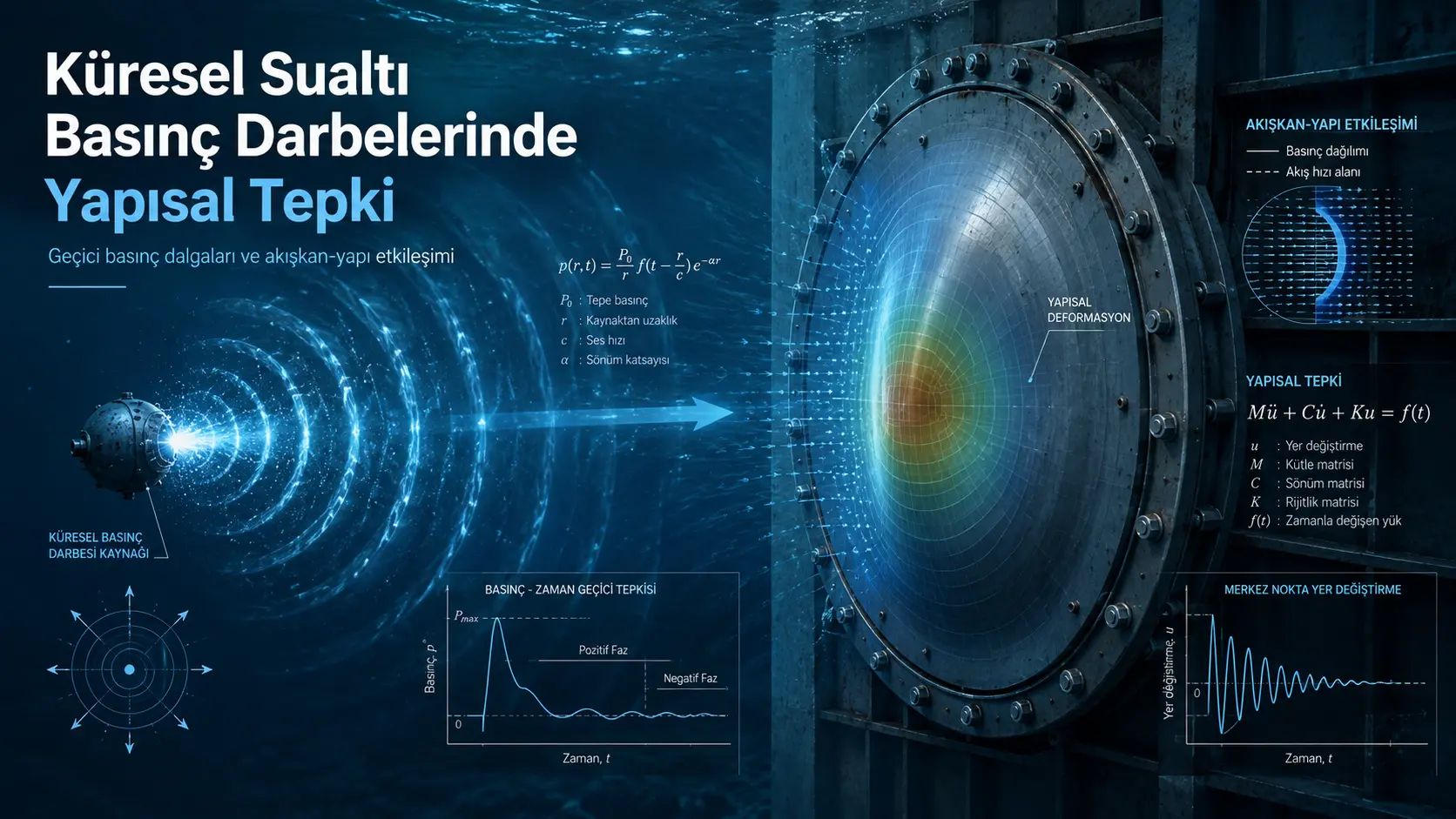
Ин таҳқиқот посухи сохторҳои монанди плитаҳои пуштибонии ҳавоӣ ва пуштибонии обиро ба pulse-ҳои фишори гузарои зериобии сферикӣ бо ҳалли аналитикии шакли пӯшида баррасӣ кардааст. Researchers сохторро бо системаҳои lumped-mass ва spring–mass-и як дараҷаи озодӣ намояндагӣ карда, solution-ҳоро бо fully coupled DYSMAS fluid–structure interaction simulations муқоиса кардаанд, ки паҳншавии 4,2 gram spherical TNT charge-ро дар conical shock tube-и пур аз об model мекунад. Spring–mass model peak transmitted pressure-ро дар water-backed systems дар ҳамаи validation cases бо хатои камтар аз %5,5 ва peak plate velocity-ро дар air-backed systems бо хатои камтар аз %16 пешгӯӣ кардааст. Бо вуҷуди ин, model reduced-order approach мебошад, ки spatial bending-и real plate, higher vibration modes, cavitation, fluid–structure separation ва full acoustic radiation field-ро ҳал намекунад.
Main conclusion-и research ин аст, ки spherical-wave geometry detail-и secondary дар structural response нест. Дар spherical waves pressure ва fluid-particle velocity дар same phase нестанд; component-е, ки “afterflow” номида мешавад, метавонад fluid motion ва energy exchange between structure and fluid-ро пас аз гузаштани pressure front ҳам идома диҳад. Study нишон медиҳад, ки parameters-и α representing fluid loading, β representing spherical spreading and afterflow, ва γ representing pulse duration якҷоя vibration, damping ва resonance regimes-ро муайян мекунанд. Plane-wave assumption ба limit-и β = 0 мувофиқ аст; бо афзоиши β predictions-и plane ва spherical models ба таври равшан аз ҳам ҷудо мешаванд.
Аз нигоҳи Туркия: Approach-и study метавонад ҳамчун analysis framework барои ship and submarine structures, pressure hulls of underwater vehicles, offshore energy facilities, underwater pipelines, pressure pulses in closed fluid systems ва preliminary design of underwater infrastructure against transient hydrodynamic loads дар Туркия мутобиқ карда шавад. Аммо барои materials, geometry, boundary conditions, water depth ва loading scenarios-и истифодашаванда дар Туркия, model бояд бо local experiments, more detailed finite-element/fluid models ва measured pressure data validate шавад. Азбаски research platform-и баҳрии сохташуда дар Туркия, domestic material, real field event ё Turkey-specific safety and cost outcomes-ро баррасӣ накардааст, direct performance ё strength conclusion барои кишвар бароварда намешавад.
Саволи асосии таҳқиқот чист?
Underwater transient pressure waves метавонанд аз underwater explosions, implosion of structures, water hammer, structural vibrations ва collapse of gas cavities ба вуҷуд оянд. Вақте ин waves ба plate ё pressure boundary мерасанд, structure ҳаракат мекунад, қисми wave reflected мешавад ва агар structure бо water surrounded бошад, pressure component ба тарафи дигар transmitted мешавад.
Қисми зиёди previous analytical studies wave front-ро planar assumed кардаанд. Ин assumption барои far field ё very large radius of curvature useful буда метавонад; аммо дар finite-radius waves relatively close to source pressure front spherical аст. Дар spherical wave phase difference between pressure and particle velocity ба вуҷуд меояд ва temporarily stored energy дар fluid afterflow-ро ҳосил мекунад.
Main question чунин аст: Spherical spreading ва afterflow vibration, damping, resonance, plate velocity ва interface pressure transmitted to opposite side-и air- ё water-backed structures-ро чӣ гуна тағйир медиҳанд?
Approach-и study ба literature
Study four closed-form models developed кардааст:
- Water-backed spring–mass system,
- Air-backed spring–mass system,
- Water-backed lumped-mass system,
- Air-backed lumped-mass system.
Spring–mass model ҳам inertia-и structure ва ҳам equivalent stiffness-ро дар бар мегирад. Lumped-mass model stiffness-ро нодида гирифта, only inertial response-ро considers. Research нишон медиҳад, ки two approaches танҳо дар certain loading ва natural-frequency conditions results-и close медиҳанд.
Air- ва water-backed structures дар Figure 1 чиро represent мекунанд?
Дар Figure 1 spherical pressure wave through water toward circular plate moves. Дар air-backed case, because air behind plate, water pressure transmitted to opposite side neglected мешавад. Дар water-backed case, water дар both sides of plate вуҷуд дорад ва additional fluid–structure interaction байни moving plate ва water behind it пайдо мешавад.
Structure бо rigid element having mass per unit area ва equivalent spring represented шудааст:
\[ m = \rho_s h \]
Here m structural mass per unit area in kg/m², ρs density of structural material in kg/m³, ва h plate thickness in meters-ро нишон медиҳад.
Equation of motion of spring–mass system:
\[ \frac{d^2w}{dt^2}+\mu^2w=\frac{P_{total}}{m} \]
w one-dimensional displacement at plate center, μ natural-frequency parameter of structure in air, Ptotal net pressure acting on plate, ва m mass per unit area-ро represent мекунад. Model spatially varying bending of real plate-ро ба single motion coordinate reduce мекунад. Bending stiffness, geometry ва edge conditions ба single equivalent spring term embedded шудаанд.
Model кадом physical details-ро дар бар намегирад?
Аз сабаби single-degree-of-freedom reduction, model directly solve намекунад:
- Spatial deformation distribution over plate surface,
- Multiple bending and vibration modes,
- Elastic waves through plate thickness,
- Local stress and deformation at edges,
- Plastic deformation or damage,
- Cavitation and fluid–structure separation,
- Full three-dimensional acoustic radiation field generated by structure
. Therefore results are reduced representation of dominant temporal system response, not detailed local stress or damage prediction.
Why is particle velocity different in spherical wave?
Fluid-particle velocity in spherical pressure wave is defined by two components:
\[ v=\frac{P}{\rho_f c_f}+\frac{1}{\rho_f R}\int_0^t P\,dt \]
Here:
- v, fluid-particle velocity, m/s;
- P, acoustic pressure, Pa;
- ρf, fluid density, kg/m³;
- cf, speed of sound in fluid, m/s;
- R, wave radius or distance between pressure source and structure, m;
- t, time, s
defined мешаванд.
First term represents acoustic energy radiating outward from source. Second integral term is afterflow. In plane-wave limit, because R becomes very large, this second term becomes small. In finite-radius spherical wave, afterflow can continue fluid motion even after pressure has decayed, altering energy exchange between structure and fluid.
Reflected and transmitted pressure mean what?
In water-backed system net pressure acting on plate:
\[ P_{total}=P_i+P_r-P_t \]
is written. Pi is incident, Pr reflected, and Pt transmitted pressure component.
“Reflected” and “transmitted” pressures in study are not full spatial acoustic-wave fields. They are reduced interface components obtained from velocity and pressure continuity at fluid–structure interface at plate center. Model does not solve motion of structure as new spherical acoustic source.
Velocity continuity at interface in water-backed case is:
\[ \frac{dw}{dt}=v_i-v_r=v_t \]
With simplification of these relations, net pressure for water-backed structure is obtained as:
\[ P_{total}=2P_r \]
.
How is incident pressure pulse modeled?
Spherical pressure wave generated at source is evaluated at constant R distance when it reaches structure location:
\[ P_i=\frac{P_{mag}}{R}\exp\left(-\frac{t}{n}\right) \]
When Pmag/R is combined as initial interface pressure P0:
\[ P_i=P_0\exp\left(-\frac{t}{n}\right) \]
is obtained. P0 denotes initial magnitude of pressure pulse at structure, and n exponential-decay time constant in seconds. This approach assumes pressure decays exponentially in time.
Three dimensionless parameters mean what?
For water-backed spring–mass system three basic dimensionless parameters are defined:
\[ \alpha=\frac{2\rho_f c_f}{\mu m} \]
\[ \beta=\frac{c_f}{\mu R} \]
\[ \gamma=\mu n \]
| Parameter | Physical meaning | Small value | Large value |
|---|---|---|---|
| α | Ratio of fluid acoustic impedance to structural inertia and stiffness | Response dominated by structural dynamics | Response dominated by fluid loading and added fluid mass |
| β | Ratio of spherical-spreading/afterflow time scale to structural natural frequency | Locally plane wave, weak afterflow | Pronounced spherical curvature and strong afterflow |
| γ | Ratio of pressure-pulse duration to structural-response time scale | Short-duration impulsive loading | Slower or quasi-static loading |
In air-backed case, because only one side of plate contacts water, factor 2 in α is absent:
\[ \alpha_{air}=\frac{\rho_f c_f}{\mu m} \]
This difference means water-backed system experiences stronger fluid loading for same physical structure and fluid.
How is natural frequency calculated?
Natural-frequency parameter of fully clamped circular plate is calculated using classical plate theory:
\[ \mu=\frac{\lambda_{mn}^2}{a^2}\sqrt{\frac{D}{m}} \]
\[ D=\frac{Eh^3}{12(1-\nu^2)} \]
Here λmn is dimensionless eigenvalue dependent on vibration mode, a plate radius, D bending stiffness, E elastic modulus, h thickness, and ν Poisson ratio.
Notation warning: Equation gives μ in angular natural-frequency form. Text later mentions conversion f = μ/(2π), but column in Table 1 is labeled “μ (Hz)” and states these values are used directly in model. This Hz-versus-rad/s notation difference is source inconsistency requiring clarification when model is reimplemented.
How were oscillatory and nonoscillatory responses separated?
Pressure equation of water-backed spring–mass system becomes third-order linear differential equation. Characteristic roots of homogeneous solution depend on α and β:
- If one real root and two complex-conjugate roots occur, system is considered underdamped or oscillatory.
- If all three roots are real, system is considered overdamped or nonoscillatory.
There is no separate structural damping term in study’s equation of motion. “Damping” visible in graphs comes from effect of fluid–structure coupling on characteristic roots. Oscillation amplitude can decrease as energy transfers to fluid; this does not mean internal viscous or structural damping was included in model.
In Figure 5 only limited region of α-β plane was overdamped. According to study, highest β at which overdamped response can occur is approximately 0,19. As β grows, afterflow can sustain fluid motion after pressure pulse and support structural oscillation.
Text defines α = 5 and β = 0,04 system as overdamped, and α = 5 and β = 0,06 as underdamped. However, in Figure 5(b), color of oscillatory curve appears reversed relative to “oscillatory/nonoscillatory” legend colors. Considering text, parameters and curve behavior together, a legend color-matching error is likely.
How did α and β change vibration frequency?
Contour maps in Figure 6 show that in underdamped region both vibration frequency and decay rate increase as α and β increase. Increasing α represents stronger fluid effect and added fluid mass relative to structure. Increasing β strengthens afterflow and sustained fluid motion around structure.
Study gives two examples:
- For α = 0,1 and β = 1,6, dimensionless damping ratio is approximately 0,013. Response continues oscillating for long time.
- For α = 1,4 and β = 0,27, damping ratio approaches approximately 1. Transmitted pressure approaches zero after about one oscillation.
Although second system mathematically lies in underdamped region with complex roots, response resembles overdamped system because of strong fluid damping.
How is resonance defined in study?
Resonance is not defined as classical steady-state resonance under periodic continuous harmonic load, but as denominator of a particular-solution coefficient in analytical solution approaching zero. Basic conditions are:
\[ \alpha=\frac{1+\gamma^2}{\gamma}-\beta(1+\gamma^2) \]
\[ \beta=\frac{1}{\gamma}-\frac{\alpha}{\gamma^2+1} \]
\[ \beta\gamma^3-\gamma^2+(\alpha+\beta)\gamma-1=0 \]
Certain α, β and γ combinations match pressure-pulse time scale with natural-response scale of reduced system, causing analytical solution to grow very large or unbounded. But this “unbounded response” is mathematical singularity of linear single-mode ideal model. In real structures plasticity, geometric nonlinearity, damage, cavitation, material damping and finite energy limit growth.
Examples in study:
- For β = 1 and γ = 0,1, pronounced resonance peak occurs when α is approximately 9,09.
- For α = 2 and γ = 0,1, resonance is obtained when β is approximately 8,02.
- For α = 1 and β = 1, analytical resonance occurs at γ approximately 0,56.
- In plane-wave example α = 1 and β = 0, no positive γ value produces resonance.
Because γ equation is cubic, more than one positive mathematical resonance root can occur for same α-β combination. These correspond to different pressure-decay durations effectively exciting same reduced system.
Why did plane and spherical wave models diverge?
β parameter contains wave radius:
\[ \beta=\frac{c_f}{\mu R} \]
As R grows, β approaches zero and spherical model tends to plane-wave limit. In plane wave, when α > 2 solution is always overdamped. In spherical model, even if α > 2, sufficiently large β can move system into oscillatory region.
Figure 9 shows ratio of maximum transmitted pressure of spherical and plane models. When β is small, two approaches are close. As β rises, afterflow strengthens and pressure predictions of two models diverge markedly. This result shows that automatically assuming plane wave for finite-radius or near-field pressure pulses can change vibration and transmission predictions.
How was numerical validation set up?
Analytical solutions were compared with fully coupled fluid–structure interaction models in Dynamic System Mechanics Advanced Simulation (DYSMAS). DYSMAS uses:
- Eulerian Gemini solver for fluid,
- Lagrangian ParaDyn solver for structure,
- Standard coupling interface between two domains
.
Gemini uses high-order Godunov-based method for shock-wave propagation in compressible inviscid fluids. Numerical model jointly simulated explosive reaction, pressure-wave propagation and interaction between wave front and target plate.
Conical shock-tube model
Figure 2 shows numerical replica of conical shock tube at Naval Undersea Warfare Center Division Newport. Tube is horizontal, water-filled and has four-section configuration with internal cone angle 2,6°:
- Explosive section,
- Conical section,
- Target plate,
- Water- or air-backed rear section.
| Numerical model feature | Value or definition |
|---|---|
| Explosive | 4,2 g spherical TNT |
| Explosive-to-target distance | 524 cm |
| Target-plate radius | 12,7 cm |
| Euler domain | 535 cm × 13 cm × 13 cm |
| Selected fluid cell | 0,15 cm |
| Total number of cells | Approximately 90,415 million |
| Structural element size | 3 mm |
| Shell element | Hughes-Liu, five integration points through thickness |
| Target boundary condition | Fully clamped |
| Target material model | Linear elastic and isotropic |
| Water density | 1000 kg/m³ |
| Sound speed in water | 1480 m/s |
| Water equation | Tillotson equation of state |
| Air equation | Gamma-law equation of state |
| Explosive equation | Jones-Wilkins-Lee equation of state |
Model used quarter symmetry in vertical and out-of-plane directions to reduce computational load. Walls of conical tube were modeled rigid, with only target plate deformable. This isolated target response by excluding deformation of surrounding structure.
How was incident pressure pulse extracted?
First simulation without target plate was run. From free-field pressure at target location:
- Initial pressure 24,1 MPa,
- Exponential decay time 0,5 ms
were identified. These values were used to form input pulse in analytical model:
\[ P_i=24{,}1\,\text{MPa}\,\exp\left(-\frac{t}{0{,}5\,\text{ms}}\right) \]
. Figure 3(a) shows this exponential curve represents general decay of numerical pressure history but not local fluctuations in simulation.
Was mesh convergence sufficient?
To ensure fluid cell size did not determine result, three simulations were run with 0,30; 0,15 and 0,05 cm cells. Comparison was done for water-backed steel plate of thickness 0,3175 cm.
| Comparison | Result |
|---|---|
| Peak transmitted-pressure difference between 0,15 cm and 0,05 cm mesh | %1,1 |
| Total-impulse difference between 0,15 cm and 0,05 cm mesh | %0,1 |
| Geers magnitude error | 0,0004 |
| Geers phase error | 0,0037 |
| Geers combined error | 0,0037 |
Based on these results 0,15 cm cell size was considered sufficient for main simulations.
What do Geers error metrics show?
Geers error metrics were used to compare not only peak value but full waveform of two time-dependent signals:
\[ G_M=\sqrt{\frac{\sum c_i^2}{\sum m_i^2}}-1 \]
\[ G_P=1-\frac{\sum m_i c_i}{\sqrt{\sum c_i^2}\sqrt{\sum m_i^2}} \]
\[ G_C=\sqrt{G_M^2+G_P^2} \]
GM indicates magnitude difference, GP waveform and phase difference, and GC combined value. Values close to zero correspond to stronger agreement between signals.
Validation of water-backed model
Seven water-backed polycarbonate and steel plate cases were modeled to cover broad α-β parameter range. Analytical-model parameters were not fitted to numerical results; they were calculated independently from material, geometry and input pulse.
| Validation metric | Result obtained |
|---|---|
| Peak transmitted-pressure error | %5,32 or lower in all cases |
| Total pressure-impulse error | %7,95 or lower in all cases |
| Average impulse error | %6,63 |
| Geers phase error | Below 0,01 |
| Geers magnitude error | About below 0,064 in absolute value |
| Geers combined error | Below 0,064 |
Lowest peak-pressure error was %0,17 for polycarbonate plate thickness 0,3175 cm; highest was %5,32 for steel plate thickness 0,9525 cm.
Figure 4(a) shows analytical and numerical pressures have similar decay trend for best-matching polycarbonate case. In Figure 4(b), although numerical curve for thick steel plate has more pronounced oscillations and late-time differences, analytical model preserves overall magnitude and decay trend.
Validation of air-backed model
For air-backed system, peak plate velocity and final displacement were compared instead of water pressure transmitted to opposite side.
| Case | Analytical peak velocity | Numerical peak velocity | Peak-velocity error | Final-displacement error |
|---|---|---|---|---|
| 0,3175 cm steel | 27,24 m/s | 32,18 m/s | %15,35 | %2,00 |
| 0,635 cm polycarbonate | 29,06 m/s | 28,55 m/s | %1,79 | %1,62 |
| 0,635 cm steel | 25,32 m/s | 28,24 m/s | %10,33 | %9,21 |
In three cases phase error stayed around or below 0,005; combined error stayed around or below 0,08. Although analytical model did not capture peak magnitude with same accuracy in every case, it qualitatively represented rise time, general magnitude and decay trend of velocity.
Why did analytical and numerical results not overlap exactly?
Main reasons for differences between DYSMAS model and reduced solution are:
- In analytical model plate is a single rigid mass and equivalent spring.
- Spatial bending and higher vibration modes are absent.
- Density changes and cavitation visible in numerical model are absent in analytical model.
- Separation between fluid and plate is neglected.
- Particle velocity is idealized as linear spherical acoustic wave.
- Reflected and transmitted pressure are interface values at plate center rather than full radiation field.
- Numerical model includes local shock-wave fluctuations while analytical input is single exponential curve.
When can transmitted pressure decrease in water-backed structures?
Figure 10 shows high- and low-transmission bands in α-β plane for γ = 0,5. At small α and large β, structural parameters dominate fluid loading and reflected pressure may approach incident pressure because of strong afterflow. Then interface pressure transmitted to opposite side decreases.
For example, at α = 0,1, β = 10 and γ = 0,5, incident and reflected pressures are close and transmitted pressure is calculated near zero. Conversely at α = 41,5, β = 2,4 and γ = 0,5, reflected pressure decreases and transmitted pressure grows.
This does not mean a real protective plate completely blocks pressure. Values are mathematical behavior of reduced interface model under specific dimensionless parameters.
Difference between air- and water-backed structures
When same dimensionless α, β and γ values are used, vibration frequency, phase and damping regime of air- and water-backed systems follow same mathematical structure. In study comparison dimensionless velocity amplitude of air-backed system was twice water-backed value.
But in real dimensional systems α values are not equal for same structure and same fluid. In water-backed structure, fluid loading is stronger because water acts from both sides. This can change:
- Amplitude,
- Vibration frequency,
- Phase,
- Damping,
- Resonance region,
- Whether response is underdamped or overdamped
. Therefore real air- and water-backed structures should be compared not only using equal dimensionless parameters but their dimensional physical values.
When did lumped-mass model become inadequate?
Lumped-mass approach assumes structural stiffness is zero:
\[ \frac{d^2w}{dt^2}=\frac{P_{total}}{m} \]
Spring–mass and lumped-mass models gave similar results when natural frequency was very small. In this case significant restoring-spring effect does not develop during loading duration and response is inertia-dominated.
As natural frequency increased, spring–mass model produced lower transmitted pressures and two solutions diverged. One important conclusion is that simply increasing mass per unit area does not make lumped-mass assumption valid. Even as mass approaches infinity, spring–mass system retains restoring term from natural frequency; lumped-mass model has no such mechanism.
Strengths of study
- Spherical-wave and afterflow effects are included in closed-form analytical solutions.
- Four different structural idealizations for air- and water-backed conditions are treated in one framework.
- Model parameters are compared without post-fitting to numerical results.
- Seven water-backed and three air-backed cases cover broad α-β range.
- Fully coupled numerical model with more than 90 million cells is used.
- Mesh convergence is tested using peak value, impulse and full time history.
- Error evaluation is based not only on peaks but also Geers magnitude and phase metrics.
- Validity regions of plane/spherical and lumped-mass/spring–mass assumptions are compared.
Limitations of study
- Study is a preprint not peer reviewed.
- No new physical experiment was conducted.
- Validation is against numerical software previously tested experimentally elsewhere; analytical solution is not directly tested against measurement data.
- Plate is reduced to one degree of freedom.
- Plastic deformation, damage and fracture are not modeled.
- Cavitation and fluid–structure separation are absent from analytical solution.
- Loading is represented by one exponential pressure pulse.
- Full three-dimensional reflected and radiated acoustic field is not solved.
- Unbounded resonance growth is not physical; it is linear-model singularity.
- Use of natural frequency in Hz or rad/s is not fully clear in source.
- Possible color-matching issue exists between legend and curve behavior in Figure 5(b).
- Overdamped region was not examined in numerical validation because fixed distance of conical tube limits accessible β range.
- Model represents only equivalent single-mode response of circular fully clamped targets.
What does study support?
- Spherical-wave curvature and afterflow can alter structural vibration and pressure-transmission predictions.
- α and β are main parameters determining underdamped or overdamped response regime.
- γ plays important role in resonance by comparing pulse duration with structural-response time.
- Spring–mass model can represent dominant pressure and velocity trends with acceptable error in examined numerical cases.
- Plane-wave approach gives close results to spherical model only when β is small.
- High mass alone is insufficient to neglect structural stiffness.
What does study not prove?
- It does not prove damage resistance of a real ship, submarine or underwater vehicle.
- It does not show a particular plate is safe against underwater explosion.
- It does not predict material yielding, cracking, rupture or permanent deformation.
- It does not show real pressure physically becomes infinite at resonance.
- It does not give transmitted interface pressure as full far-field acoustic pressure field.
- It does not prove all waveforms can be represented by exponential-decay model.
- It does not establish validated design standard for marine structures in Turkey.
Meaning for everyday and engineering applications
Main value of study is not direct final-structure design but enabling rapid screening of dominant parameters before detailed simulation or experiment. An engineer can vary material density, thickness, natural frequency, fluid properties, wave radius and pulse duration to preliminarily assess which vibration regime system approaches.
Approach can be investigated as reduced-order screening tool for preliminary design of underwater pressure hulls, transient pressure boundaries in closed water systems, ship plating, offshore platforms, underwater pipes and shock-tube experiments. Real design decisions additionally require material nonlinearity, damage, welds and joints, three-dimensional geometry, different pressure shapes and experimental validation.
Усул ва бозёфтҳои таҳқиқот
Methodological design
| Method component | Approach applied in study |
|---|---|
| Study type | Closed-form analytical modeling and fully coupled numerical FSI validation |
| Structural idealization | Single-degree-of-freedom spring–mass and lumped mass |
| Backing conditions | Air-backed and water-backed |
| Pressure wave | Spherical, exponentially decaying transient pulse |
| Primary outputs | Reflected and transmitted interface pressure, plate velocity, displacement, vibration regime and resonance |
| Dimensionless parameters | α: FSI, β: spherical geometry/afterflow, γ: loading duration |
| Numerical software | DYSMAS; Gemini Euler solver and ParaDyn Lagrange solver |
| Explosive model | 4,2 g spherical TNT, JWL equation of state |
| Fluid | Water: 1000 kg/m³, 1480 m/s; Tillotson equation of state |
| Target | Fully clamped circular steel or polycarbonate plate of radius 12,7 cm |
| Validation cases | Seven water-backed, three air-backed structures |
| Mesh convergence | 0,30; 0,15 and 0,05 cm fluid cells |
| Error metrics | Peak value, total impulse, final displacement and Geers GM-GP-GC metrics |
| Physical experiment | Not performed in this study |
Materials and structural ranges used for validation
| Property | Polycarbonate | Steel |
|---|---|---|
| Elastic modulus | 2,3 GPa | 210 GPa |
| Density | 1200 kg/m³ | 7800 kg/m³ |
| Poisson ratio | 0,4 | 0,3 |
| Examined thicknesses | 0,158-0,952 cm | 0,3175-0,9525 cm |
| Mass per unit area range | 1,90-11,43 kg/m² | 24,77-74,30 kg/m² |
Selected numerical results from water-backed cases
| Case | Analytical peak pressure | Numerical peak pressure | Peak error | Impulse error |
|---|---|---|---|---|
| 0,3175 cm polycarbonate | 22,06 MPa | 22,02 MPa | %0,17 | %7,28 |
| 0,3175 cm steel | 20,87 MPa | 21,48 MPa | %2,84 | %6,01 |
| 0,635 cm steel | 19,66 MPa | 20,00 MPa | %1,69 | %3,16 |
| 0,9525 cm steel | 19,00 MPa | 20,07 MPa | %5,32 | %7,95 |
Main findings
- Spring–mass analytical solution predicted peak transmitted pressure in examined water-backed cases with error below %5,5.
- Total impulse error in water-backed cases was below %8, average impulse error %6,63.
- Peak plate-velocity error in air-backed cases ranged from %1,79 to %15,35.
- Final-displacement error in air-backed cases ranged from %1,62 to %9,21.
- Peak-pressure difference between 0,15 cm and 0,05 cm mesh was only %1,1.
- As β approached approximately zero, spherical and plane model results approached each other.
- As β increased, afterflow sustained oscillatory responses not predicted by plane model.
- For overdamped region to occur, β had to be smaller than approximately 0,19.
- Certain α-β-γ combinations produced resonance singularity in analytical solution.
- At same dimensionless parameters, air-backed velocity amplitude was calculated as twice water-backed amplitude.
- In real dimensional comparison, water-backed structure showed stronger fluid loading, different frequency and different damping.
- As natural frequency increased, spring–mass and lumped-mass models diverged markedly.
- Increasing mass per unit area alone did not justify neglecting stiffness.
Mechanism shown collectively by figures
Figure 3 shows exponential approximation of input pressure and mesh convergence; Figure 4 analytical–numerical time-history agreement; Figures 5 and 6 vibration and damping regimes in α-β plane. Figures 7 and 8 show resonance depends not on one parameter but narrow regions jointly created by α, β and γ.
Figure 9 shows plane and spherical wave predictions diverge as β increases. Figure 10 shows low- and high-transmission bands in water-backed systems; Figures 11 and 12 show resonance and damping should be assessed together. Figure 13 explains dimensionless similarity but dimensional physical difference between air- and water-backed conditions; Figure 14 explains validity limit of lumped-mass approach neglecting structural stiffness.
Interpretation boundary of results
Low error values show dominant temporal behavior of examined DYSMAS cases can be represented by single-degree-of-freedom analytical system. This does not mean model predicts local stress, damage, cavitation or full acoustic field in real structures with same accuracy. Analytical solution is not final certification tool replacing detailed simulation and experiments, but parameter-sensitivity and preliminary-assessment method.
Ёддошти манбаъ ва усул
Full original title of study: Response of Structures Subjected to Spherical Underwater Transient Pressure Pulses
Authors: Carlos Javier, Shyamal Kishore, Michael Galuska, Michael Papa, James LeBlanc, Helio Matos and Arun Shukla.
Author order: Preserved as given in source.
Co-first author: No equal contribution or co-first authorship information is provided.
Corresponding author: Carlos Javier. Contact address given in study is carlos.r.javier.civ@us.navy.mil.
Institution 1: Naval Undersea Warfare Center, Division Newport, 1176 Howell Street, Newport, Rhode Island 02841, USA.
Institution 2: Dynamic Photo Mechanics Laboratory, Department of Mechanical, Industrial and Systems Engineering, University of Rhode Island, Kingston, Rhode Island 02881, USA.
Official source link:Current SSRN record page
Previous SSRN version: An older record with SSRN 6571436 and DOI 10.2139/ssrn.6571436 also exists for same title. This content uses current uploaded version carrying number 7197531.
Publication platform: SSRN.
Journal: No specific peer-reviewed journal name or journal acceptance appears in this version.
Original publisher: No peer-reviewed journal publisher; study is presented on SSRN preprint platform.
Publication year: 2026.
Source type: Modeling study containing closed-form analytical solutions and fully coupled fluid–structure interaction simulations.
Peer-review status: This study is a preprint not peer reviewed; results should be read with this limitation.
Funding: Research funded by National Institute for Undersea Vehicle Technology under NIUVT Cooperative Research and Development Agreement NCRADA-NUWCDIVNPT-23-2214.
Acknowledgments: Researchers thank Robert Koch for contribution on underwater pressure-wave propagation and Elizabeth Magliula for contribution to development of study topic.
Author contributions: No separate CRediT or task-based author-contribution statement is included.
Conflict of interest: No separate conflict-of-interest or competing-interests statement appears in this version.
Data and code access: No open-data repository, model-code or reproduction-package link is provided.
Methodological boundary: Analytical solution is a single-degree-of-freedom reduced model. Spatial deformation, higher modes, plastic damage, cavitation, fluid–structure separation and full acoustic radiation field are not solved. Validation is based on DYSMAS simulations rather than new physical experiments.
Source-consistency note: Representation of natural-frequency parameter in Hz versus rad/s is not fully consistent in source. Colors of oscillatory and nonoscillatory curves in Figure 5(b) also appear reversed relative to legend. These points are stated without silently changing source text.
Ин мазмуни тоҷикӣ дар асоси scientific text, equations, tables, figures, appendices ва results-и uploaded study омода шудааст. No experimental result, field success, damage resistance, military performance, commercial applicability or safety guarantee absent from study илова нашудааст.
Шарҳ гузоред
Нишонии почтаи электронии шумо нашр намешавад. Майдонҳои ҳатмӣ бо * нишон дода шудаанд